Download
1 / 27
310 likes | 721 Views
Chap.3. Fundamentals of Inviscid, Incompressible Flow. OUTLINE. Bernoulli ’ s equation and its application Pressure coefficient Laplace ’ s equation for irrotational, incompressible flow Elementary flows Combination of elementary flows. Bernoulli ’ s equation and its application.

E N D
Chap.3 Fundamentals of Inviscid, Incompressible Flow
OUTLINE • Bernoulli’s equation and its application • Pressure coefficient • Laplace’s equation for irrotational, incompressible flow • Elementary flows • Combination of elementary flows
Bernoulli’s equation and its application • Bernoulli’s equation • Relation between pressure and velocity in an inviscid, incompressible flow. • Equation form along a streamline • If the flow is irrotational, throughout the flow
Flow in a duct • Continuity equation for quasi-one-dimensional flow in a duct • For incompressible flow
The venturi and low-speed wind tunnel • In aerodynamic application, venturi can be used to measure the velocity of inlet flow V1. • From Bernoulli’s equation:
A low-speed wind tunnel is a large venturi where the airflow is driven by a fan. • The test section flow velocity can be derived from Bernoulli’s equation
Pitto tube • Stagnation point: a point in a flow where V = 0. (ex. Point B in the figure.) • Stagnation pressure p0: pressure at a stagnation point, also called total pressure. • To measure the flight velocity of an airplane.
Pressure coefficient • Pressure coefficient is defined as where • For incompressible flow • Cp can be reduced to be in terms of velocity only.
Laplace’s equation for irrotational, incompressible flow • For incompressible flow • For irrotational flow ( is velocity potential) • Laplace’s equation • The stream function also satisfies Laplace’s equation.
Solution of Laplace’s equation • Solutions of Laplace’s equation are called harmonic functions. • Superposition principle is applicable since Laplace’s equation is linear. • A complicated flow pattern can be synthesized by adding together a number of elementary flows.
Boundary contions • Infinity boundary conditions • Wall boundary conditions (wall tangency conditions)
Uniform flow A uniform flow is a physically possible incompressible and irrotational flow. Boundary condition for Solution for Elementary flows
Boundary condition for • Solution for
Source flow • Cylindrical coordinate system is applied. • Incompressible at every point except the origin. • Irrotational at every point. • Velocity field where is the source strength, defined as the volume flow rate per unit length.
is positive for a source flow, whereas negative for a sink flow. • Solution for and
Doublet flow • A pair of source-sink with the same strength, while the distance l between each other tends to zero. • Stream function where =const. is the strength of the doublet.
Solution for and • The direction of a doublet is designated by an arrow draw form the sink to the source.
Vortex flow • A flow where all the streamlines are concentric circles, and the velocity along any circular streamline is constant. • Incompressible at every point. • Irrotational at every point except the origin.
Velocity field where is the circulation. • Solution for and
Combination of elementary flows • Superposition of a uniform flow and a source • Stream function
Velocity field • Stagnation point • The streamline goes through the stagnation point is described by =/2, shown as curve ABC.
Streamline ABC separates the fluid coming from the free stream and the fluid emanating from the source. • The entire region inside ABC could be replaced with a solid body of the same shape.
Superposition of a uniform flow and a source-sink pair • Stream function
Two stagnation points A and B are found by setting V=0. • The stagnation streamline is given by =0, i.e. which is the equation of an oval, called Rankine oval. • The region inside the oval can be replaced by a solid body with the same shape.
Nonlifting flow over a circular cylinder • Superposition of a uniform flow and a doublet • Stream function
Velocity field • The stagnation streamline is given by =0, i.e. • The stagnation streamline includes the circle described by r=R, and the entire horizontal axis through points A and B.
We can replace the flow inside the circle by a solid body. Consequently, a flow over a circular cylindrical of radius R can be synthesized by this superposition, where • The pressure distribution is symmetric about both axes. As a result, there is no net lift, as well as no net drag which makes no sense in real world.