Download
1 / 17
180 likes | 216 Views
Explore the impact of radio occultation geometry, bending angle, and signal inversion in atmospheric studies. Learn about back-propagation techniques and canonical transform methods to enhance data accuracy.

E N D
Radio Occultation and Multipath Behavior Kent Bækgaard Lauritsen Danish Meteorological Institute (DMI), Denmark 2nd GRAS SAF User Workshop, 11-13 June 2003
Outline of the Talk • Introduction • Multipath behavior • Inversion of 1-ray and multipath signals • Back-propagation • Canonical transform methods • Conclusions and outlook
Radio Occultation Geometry Impact parameter Bending angle
Radio Occultation Signal Physical signal: E, B Measured signal: u(t) u(t) = uEM + Receiver noise & tracking errors Receiver: - small noise will not cause problems - tracking errors: need to be known in order to be able to correct for them Two tracking modes: - closed loop: phase-locked loop (PLL) - open loop: raw signal
Wave Optics Simulation Example Standard atmosphere
Water Vapor and Multipath Tropics: dense water vapor layers will in general give rise to multipath propagation of radio signals Critical refraction condition: - ducting of rays Horizontal gradients: - normally, one assumes spherical symmetry in order to obtain the refractivity N(r) from (p) using the Abel transform
Inversion of 1-Ray Signal Measured signal: Doppler shift (‘wave vector’ along the t coordinate): Bending angle, (p), obtainable from (t) (using geometry) Refractivity, N(r), using the Abel transform (& spherical symmetry) Atmospheric quantities: P, T, q, …
Inversion of Multipath Signal Measured, multi-ray representation: u(t): t-representation, with caustic with 3 rays at a given time, t Map to a 1-ray representation: uz(z): z-representation with 1 ray at any given value of the ‘coordinate’ z Wave vector along the z-coordinate: Bending angle, (p), obtainable from (z) Phase space: (z, ) are new coordinates, replacing (y,ky)
Back-Propagation Method Back-propagation maps the measured field u(t) to a new field with x xB: B: known from the Green’s function for the Helmholtz equation Wave vector along the yB-coordinate: Bending angle, (p), obtainable from kB: Phase space: (yB,kB) are new coordinates in the (y,ky) phase space Does yB uniquely define the rays? - no, real and imaginary caustics may overlap - multipath tend to be reduced, thus results are slightly improved
Impact Parameter Representation Physical insight: for a spherical symmetric atmosphere, the impact parameter, p, uniquely defines a ray [Gorbunov]; with horizontal gradients the assumption will be fulfilled to a good approximation Thus, choose z = p and map the measured field to the p-representation: up(p) Mathematical physics provides the recipe for calculating up(p): whereFis a Fourier integral operator (FIO) with phase function being equal to the generating function for the canonical transform from the old to the new (p, ) coordinates; note, there are infinitely manyF’s that map to the p-representation
Canonical Transform Method Map to the 1-rayp-representation: Wave vector along the p-coordinate: Bending angle, (p), obtainable from (p):e(p) = x(p) (plus a correction when the GPS satellite is at a finite position)
Canonical Transform Method of ‘‘Type 2’’ Canonical transform (of type 1): - Gorbunov’s original CT method which involves first doing back-propagation - FIO, F, based on a canonical transform from (yB, kB) to (p, ) coordinates Canonical transform (of type 2): - CT method based on directly mapping the measured field u(t) to the p-representation, up(p) [FSI] - FIO, F2, based on a canonical transform from (t, ) to (p, ) coordinates - up(p) can be chosen to be identical to the one obtained by a CT of type 1 - GPS satellite is not assumed stationary
Conclusions and Outlook • Radio occultations and multipath behavior • Water vapor, critical refraction, receiver tracking errors • Mapping from multi-ray to 1-ray representation • Multi-ray: caustics • 1-ray: Impact parameter representation • Inversion methods • Standard methods: handle 1-ray signals • Back-propagation: can reduce multi-ray behavior • Canonical transform methods: handle multi-ray behavior • Gorbunov’s original CT & CT without back-propagation (CT of type 2) • Increased vertical resolution (about 50 m) • Improved product accuracy