Download
1 / 18
180 likes | 292 Views
S010Y: Answering Questions with Quantitative Data Class 9/III.2: Displaying Relationships Between Continuous Variables. Research Is A Partnership Of Questions And Data. S010Y: Answering Questions with Quantitative Data Class 9/III.2: Displaying Relationships Between Continuous Variables.

E N D
S010Y: Answering Questions with Quantitative DataClass 9/III.2: Displaying Relationships Between Continuous Variables Research Is A Partnership Of Questions And Data
S010Y: Answering Questions with Quantitative DataClass 9/III.2: Displaying Relationships Between Continuous Variables Here’s the codebook for the data we’ll use in this part of the module …
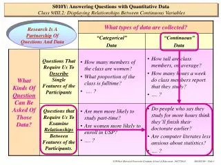
S010Y: Answering Questions with Quantitative DataClass 9/III.2: Displaying Relationships Between Continuous Variables We can use these data to address a variety of interesting research questions, including this one … Research Question: “Are high school graduation rates higher in states where there are fewer students per teacher?” • question about a potential relationshipbetweentwo continuous variables: • Statewide High-School graduation rates (HSGRADRT), • Student/Teacher ratio (STRATIO) So, in other words, I’m really asking: Are HSGRADRT and STRATIO related? How do we answer this question?
Regular data input paragraph • STATE is an “string” variable: • Values are alphabetic characters (that is, the names of the states), • We tell PC_SAS by putting a “$” symbol after the variable name in the input statement. This paragraph sorts the data in descending order of high-school graduation rate, HSGRADRT, to facilitate comparisons across states. Names the columns in the print listing with the variable labels, rather than the variable names Print out the data for inspection S010Y: Answering Questions with Quantitative DataClass 9/III.2: Displaying Relationships Between Continuous Variables I begin the analysis in Class9/Handout1 -- here’s the start of the PC-SAS program … OPTIONS Nodate Pageno=1; TITLE1 ‘S010Y: Answering Questions with Quantitative Data'; TITLE2 'Class 9/Handout 1: Displaying Relationships Between Continuous Variables'; TITLE3 'The Infamous Wallchart Data'; TITLE4 'Data in WALLCHT.txt'; *--------------------------------------------------------------------------------* Input data, name and label variables in the dataset *--------------------------------------------------------------------------------*; DATA WALLCHT; INFILE 'C:\DATA\A010Y\WALLCHT.txt'; INPUT STATE $ TCHRSAL STRATIO PPEXPEND HSGRADRT; LABEL TCHRSAL = '1988 Average Teacher Salary' STRATIO = '1988 Student/Teacher Ratio' PPEXPEND = '1988 Expenditure/Student' HSGRADRT = '1988 Statewide H.S. Graduation Rate'; *--------------------------------------------------------------------------------* Data Listing, with the States ranked in descending order by values of HSGRADRT *--------------------------------------------------------------------------------*; PROC SORT DATA=WALLCHT; BY DESCENDING HSGRADRT; PROC PRINT LABEL DATA=WALLCHT; TITLE5 'Listing of Data, in Descending Order of H.S. Graduation Rates'; VAR STATE HSGRADRT STRATIO TCHRSAL PPEXPEND;
S010Y: Answering Questions with Quantitative DataClass 9/III.2: Displaying Relationships Between Continuous Variables The data-listing produced by PC-SAS … demonstrates considerable heterogeneity on all four variables!!! 1988 Statewide 1988 1988 H.S. Student/ Average 1988 Graduation Teacher Teacher Expenditure/ STATE Rate Ratio Salary Student MN 90.9 17.1 29900 4386 ND 88.3 15.6 21660 3519 WY 88.3 14.5 27134 5051 MT 87.3 15.8 23798 4246 IA 85.8 15.6 24847 4124 NE 85.4 15.1 22683 3943 CT 84.9 13.3 33487 6230 WI 84.9 16.2 29122 4747 KS 80.2 15.4 24647 4076 OH 79.6 18.0 27606 3998 SD 79.6 15.5 19758 3249 UT 79.4 24.7 22572 2454 VT 78.7 13.9 24519 5207 PE 78.4 16.2 29177 4989 NJ 77.4 14.0 30720 6564 WV 77.3 15.2 21736 3858 AR 77.2 17.1 20340 2989 WA 77.1 20.2 28217 4164 IN 76.3 17.9 26881 3794 NV 75.8 20.2 27600 3623 IL 75.6 17.2 29663 4369 ID 75.4 20.7 22242 2667 AL 74.9 19.3 23320 2718 CO 74.7 18.0 28651 4462 ME 74.4 14.9 23425 4258 MA 74.4 13.9 30295 5471 MD 74.1 17.1 30933 5201 NH 74.1 16.0 24019 4457 MO 74.0 16.2 24709 3786 MI 73.6 19.9 32926 4692 OR 73.0 18.3 28060 4789 NM 71.9 18.9 24158 3691 DL 71.7 16.1 29573 5017 OK 71.7 16.9 21630 3093 VA 71.6 16.3 27193 4149 RI 69.8 15.0 32858 5329 TN 69.3 19.6 23785 3068 HI 69.1 21.6 28785 3916 KY 69.0 18.2 24253 3011 MS 66.9 18.8 20562 2548 NC 66.7 18.2 24900 3368 CA 65.9 22.9 33159 3840 AK 65.5 17.3 40424 7971 TX 65.3 17.3 25558 3608 SC 64.6 17.2 24403 3408 NY 62.3 15.2 34500 7151 LA 61.4 18.5 21209 3138 AZ 61.1 18.6 27388 3744 GA 61.0 18.7 26190 3434 FL 58.0 17.4 25198 4092
Here are the usual PROC UNIVARIATE commands to obtain: • Univariate summary statistics, • Stem-Leaf & Boxplots. On the WALLCHT data. • Specifies the variables for which descriptive statistics are required: • Notice that you can list both HSGRADRT and STRATIO. Implementing the ID command ensures that the cases are identified by the (alphabetic) value of the STATE variable S010Y: Answering Questions with Quantitative DataClass 9/III.2: Displaying Relationships Between Continuous Variables Then, I asked PC-SAS to provide univariate descriptive statistics on the HSGRADRT and STRATIO variables … *-------------------------------------------------------------------------* Descriptive statistics on graduation rates and student/teacher ratios *-------------------------------------------------------------------------*; PROC UNIVARIATE PLOT DATA=WALLCHT; TITLE5 'Distribution of H.S. Graduation Rates and Student/Teacher Ratios'; VAR HSGRADRT STRATIO; ID STATE;
S010Y: Answering Questions with Quantitative DataClass 9/III.2: Displaying Relationships Between Continuous Variables The UNIVARIATE Procedure Variable: HSGRADRT (1988 Statewide H.S. Graduation Rate) N 50 Sum Weights 50 Mean 74.276 Sum Observations 3713.8 Std Deviation 7.83317279 Variance 61.3585959 Skewness 0.06455725 Kurtosis -0.3745981 Basic Statistical Measures Location Variability Mean 74.27600 Std Deviation 7.83317 Median 74.40000 Variance 61.35860 Mode 71.70000 Range 32.90000 Interquartile Range 9.60000 Quantile Estimate 100% Max 90.90 99% 90.90 95% 88.30 90% 85.60 75% Q3 78.70 50% Median 74.40 25% Q1 69.10 10% 63.45 5% 61.10 1% 58.00 0% Min 58.00 Extreme Observations ----------Lowest--------- ---------Highest--------- Value STATE Obs Value STATE Obs 58.0 FL 50 85.8 IA 5 61.0 GA 49 87.3 MT 4 61.1 AZ 48 88.3 ND 2 61.4 LA 47 88.3 WY 3 62.3 NY 46 90.9 MN 1 Here are the univariate descriptive statistics for continuous variable HSGRADRT … Stem Leaf # Boxplot 90 9 1 | 88 33 2 | 86 3 1 | 84 9948 4 | 82 | 80 2 1 | 78 47466 5 +-----+ 76 31234 5 | | 74 0114479468 10 *--+--* 72 06 2 | | 70 6779 4 | | 68 0138 4 +-----+ 66 79 2 | 64 6359 4 | 62 3 1 | 60 014 3 | 58 0 1 | ----+----+----+ Can you interpret these univariate descriptive statistics?
S010Y: Answering Questions with Quantitative DataClass 9/III.2: Displaying Relationships Between Continuous Variables The UNIVARIATE Procedure Variable: STRATIO (1988 Student/Teacher Ratio) N 50 Sum Weights 50 Mean 17.314 Sum Observations 865.7 Std Deviation 2.34041772 Variance 5.4775551 Skewness 0.83218447 Kurtosis 1.08658239 Basic Statistical Measures Location Variability Mean 17.31400 Std Deviation 2.34042 Median 17.15000 Variance 5.47756 Mode 16.20000 Range 11.40000 Interquartile Range 3.00000 Quantile Estimate 100% Max 24.70 99% 24.70 95% 21.60 90% 20.20 75% Q3 18.60 50% Median 17.15 25% Q1 15.60 10% 14.70 5% 13.90 1% 13.30 0% Min 13.30 Extreme Observations ----------Lowest--------- ---------Highest--------- Value STATE Obs Value STATE Obs 13.3 CT 7 20.2 NV 20 13.9 MA 26 20.7 ID 22 13.9 VT 13 21.6 HI 38 14.0 NJ 15 22.9 CA 42 14.5 WY 3 24.7 UT 12 Here are the univariate descriptive statistics on continuous variable STRATIO ….. Stem Leaf # Boxplot 24 7 1 0 24 23 23 22 9 1 | 22 | 21 6 1 | 21 | 20 7 1 | 20 22 2 | 19 69 2 | 19 3 1 | 18 56789 5 +-----+ 18 00223 5 | | 17 9 1 | | 17 11122334 8 *--+--* 16 9 1 | | 16 012223 6 | | 15 5668 4 +-----+ 15 01224 5 | 14 59 2 | 14 0 1 | 13 99 2 | 13 3 1 | ----+----+----+ Can you interpret these univariate descriptive statistics?
PROC PLOT is a PC_SAS routine that produces bivariatescatter-plots of continuous variables Choose an appropriate scaling for the vertical axis. Plot HSGRADRT on the vertical axis versus STRATIO on the horizontal axis Choose an appropriate scaling for the horizontal axis. S010Y: Answering Questions with Quantitative DataClass 9/III.2: Displaying Relationships Between Continuous Variables But, are HSGRADRT and STRATIO related?To address this question, we must displayHSGRADRTandSTRATIOsimultaneously in a bivariate scatterplot … *------------------------------------------------------------------------* Displaying the relationship between HSGRADRT and STRATIO *------------------------------------------------------------------------*; PROC PLOT DATA=WALLCHT; TITLE5 'Plot of H.S. Graduation Rates against Student/Teacher Ratios'; PLOT HSGRADRT*STRATIO / HAXIS = 10 TO 25 BY 5 VAXIS = 50 TO 100 BY 10; RUN;
Vertical axis (or ordinate), displays the value of “outcome,” HSGRADRT • Points on the scatterplot – like symbol “A” --represent each State, and display values of outcome HSGRADRT & predictor STRATIO simultaneously. • In Ohio, HSGRADRT=79.6,STRATIO=18.0. OHIO 79.6 ? Horizontal axis (or abscissa), displays the value of “predictor,” STRATIO 18.0 S010Y: Answering Questions with Quantitative DataClass 9/III.2: Displaying Relationships Between Continuous Variables Here’s a bivariate plot of HSGRADRT versus STRATIO … 1 100 ˆ 9 ‚ 8 ‚ 8 ‚ ‚ S ‚ t ‚ A a 90 ˆ t ‚ A A e ‚ A w ‚ A A i ‚ A A d ‚ e ‚ 80 ˆ B A A H ‚ A A . ‚ A A A A S ‚ A A A A . ‚ A A AA A A A A ‚ A G ‚ AA A A r 70 ˆ A A a ‚ A A d ‚ A A u ‚ B A a ‚ A t ‚ A i ‚ AB o 60 ˆ n ‚ A ‚ R ‚ a ‚ t ‚ e ‚ 50 ˆ Šƒƒˆƒƒƒƒƒƒƒƒƒƒƒƒƒƒƒƒƒƒƒƒƒˆƒƒƒƒƒƒƒƒƒƒƒƒƒƒƒƒƒƒƒƒƒˆƒƒƒƒƒƒƒƒƒƒƒƒƒƒƒƒƒƒƒƒƒˆƒƒ 10 15 20 25 1988 Student/Teacher Ratio
Is this the case here? S010Y: Answering Questions with Quantitative DataClass 9/III.2: Displaying Relationships Between Continuous Variables And, how can we tell if HSGRADRT and STRATIO are related? 1 100 ˆ 9 ‚ 8 ‚ 8 ‚ ‚ S ‚ t ‚ A a 90 ˆ t ‚ A A e ‚ A w ‚ A A i ‚ A A d ‚ e ‚ 80 ˆ B A A H ‚ A A . ‚ A A A A S ‚ A A A A . ‚ A A AA A A A A ‚ A G ‚ AA A A r 70 ˆ A A a ‚ A A d ‚ A A u ‚ B A a ‚ A t ‚ A i ‚ AB o 60 ˆ n ‚ A ‚ R ‚ a ‚ t ‚ e ‚ 50 ˆ Šƒƒˆƒƒƒƒƒƒƒƒƒƒƒƒƒƒƒƒƒƒƒƒƒˆƒƒƒƒƒƒƒƒƒƒƒƒƒƒƒƒƒƒƒƒƒˆƒƒƒƒƒƒƒƒƒƒƒƒƒƒƒƒƒƒƒƒƒˆƒƒ 10 15 20 25 1988 Student/Teacher Ratio Two variables are related if…
You be the judge? S010Y: Answering Questions with Quantitative DataClass 9/III.2: Displaying Relationships Between Continuous Variables What kind of line, curve or other construction bestsummarizes the observed relationship between HSGRADRT and STRATIO? 1 100 ˆ 9 ‚ 8 ‚ 8 ‚ ‚ S ‚ t ‚ A a 90 ˆ t ‚ A A e ‚ A w ‚ A A i ‚ A A d ‚ e ‚ 80 ˆ B A A H ‚ A A . ‚ A A A A S ‚ A A A A . ‚ A A AA A A A A ‚ A G ‚ AA A A r 70 ˆ A A a ‚ A A d ‚ A A u ‚ B A a ‚ A t ‚ A i ‚ AB o 60 ˆ n ‚ A ‚ R ‚ a ‚ t ‚ e ‚ 50 ˆ Šƒƒˆƒƒƒƒƒƒƒƒƒƒƒƒƒƒƒƒƒƒƒƒƒˆƒƒƒƒƒƒƒƒƒƒƒƒƒƒƒƒƒƒƒƒƒˆƒƒƒƒƒƒƒƒƒƒƒƒƒƒƒƒƒƒƒƒƒˆƒƒ 10 15 20 25 1988 Student/Teacher Ratio
What kind of line, curve or other construction bestsummarizes the observed relationship between HSGRADRT and STRATIO? 1 100 ˆ 9 ‚ 8 ‚ 8 ‚ ‚ S ‚ t ‚ A a 90 ˆ t ‚ A A e ‚ A w ‚ A A i ‚ A A d ‚ e ‚ 80 ˆ B A A H ‚ A A . ‚ A AAA S ‚ A AAA . ‚ A A AA A AAA ‚ A G ‚ AA A A r 70 ˆ A A a ‚ A A d ‚ A A u ‚ B A a ‚ A t ‚ A i ‚ AB o 60 ˆ n ‚ A ‚ R ‚ a ‚ t ‚ e ‚ 50 ˆ Šƒƒˆƒƒƒƒƒƒƒƒƒƒƒƒƒƒƒƒƒƒƒƒƒˆƒƒƒƒƒƒƒƒƒƒƒƒƒƒƒƒƒƒƒƒƒˆƒƒƒƒƒƒƒƒƒƒƒƒƒƒƒƒƒƒƒƒƒˆƒƒ 10 15 20 25 1988 Student/Teacher Ratio S010Y : Answering Questions with Quantitative DataClass 10&11/III.3: Summarizing Relationships Between Continuous Variables Here’s My Best Guess! It was obtained by a mystery process called “Ordinary Least-Squares (OLS) Regression Analysis.”
Here are the usual data input statements Here are the PC-SASregressionanalysis commands – we dissect them in detail on the next slide Creates another scatterplot of the data for use later Of course, you can also get PC-SAS to tell you where the OLS-fitted regression line is … OPTIONS Nodate Pageno=1; TITLE1 ‘S010Y: Answering Questions with Quantitative Data'; TITLE2 'Class 10/Handout 1: Summarizing Relationships Between Continuous Variables'; TITLE3 'The Infamous Wallchart Data'; TITLE4 'Data in WALLCHT.txt'; *--------------------------------------------------------------------------------* Input data, name and label variables in the dataset *--------------------------------------------------------------------------------*; DATA WALLCHT; INFILE 'C:\DATA\A010Y\WALLCHT.txt'; INPUT STATE $ TCHRSAL STRATIO PPEXPEND HSGRADRT; LABEL TCHRSAL = '1988 Average Teacher Salary' STRATIO = '1988 Student/Teacher Ratio' PPEXPEND = '1988 Expenditure/Student' HSGRADRT = '1988 Statewide H.S. Graduation Rate'; *--------------------------------------------------------------------------------* Using regression analysis to summarize the relationship of HSGRADRT and STRATIO *--------------------------------------------------------------------------------*; PROC REG DATA=WALLCHT; TITLE5 'OLS Regression of H.S. Graduation Rate on Student/Teacher Ratio'; MODEL HSGRADRT = STRATIO; *--------------------------------------------------------------------------------* Plotting the relationship between HSGRADRT and STRATIO *--------------------------------------------------------------------------------*; PROC PLOT DATA=WALLCHT; TITLE5 'Plot of H.S. Graduation Rates against Student/Teacher Ratios'; PLOT HSGRADRT*STRATIO / HAXIS = 10 TO 25 BY 5 VAXIS = 50 TO 100 BY 10; RUN; S010Y : Answering Questions with Quantitative DataClass 10&11/III.3: Summarizing Relationships Between Continuous Variables
PROC REG is the command in PC-SAS that requests an OLS Regression Analysis You request an OLS Regression Analysis by specifying a “Regression Model” that identifies the “Outcome” and the “Predictor(s)” to include in the analysis: Model HSGRADRT = STRATIO You identify the outcome variable (HSGRADRT) by placing it to the leftof the “equals” sign, in the MODEL statement You identify the predictor variable (STRATIO) by placing it to the rightof the “equals” sign, in the MODEL statement Here’s the part of the PC_SAS program that deals specifically with the OLSRegression Analysisof the HSGRADRT versus STRATIO relationship … *--------------------------------------------------------------------------------* Using regression analysis to summarize the relationship of HSGRADRT and STRATIO *--------------------------------------------------------------------------------*; PROC REG DATA=WALLCHT; TITLE5 'OLS Regression of H.S. Graduation Rate on Student/Teacher Ratio'; MODEL HSGRADRT = STRATIO; S010Y : Answering Questions with Quantitative DataClass 10&11/III.3: Summarizing Relationships Between Continuous Variables
Ignore this part of the output. When you go on to S030, you’ll learn what it all means This is the major part of the “regression analysis” output. I unpack it on the next several slides Here’s output from the OLS Regression AnalysisofOutcome HSGRADRT on PredictorSTRATIO….. The REG Procedure Model: MODEL1 Dependent Variable: HSGRADRT 1988 Statewide H.S. Graduation Rate Analysis of Variance Sum of Mean Source DF Squares Square F Value Pr > F Model 1 337.52168 337.52168 6.07 0.0174 Error 48 2669.04952 55.60520 Corrected Total 49 3006.57120 Root MSE 7.45689 R-Square 0.1123 Dependent Mean 74.27600 Adj R-Sq 0.0938 Coeff Var 10.03943 Parameter Estimates Parameter Standard Variable Label DF Estimate Error t Value Intercept Intercept 1 93.69187 7.95093 11.78 STRATIO 1988 Student/Teacher Ratio 1 -1.12140 0.45516 -2.46 Parameter Estimates Variable Label DF Pr > |t| Intercept Intercept 1 <.0001 STRATIO 1988 Student/Teacher Ratio 1 0.0174 S010Y : Answering Questions with Quantitative DataClass 10&11/III.3: Summarizing Relationships Between Continuous Variables
These “Parameter Estimates” tell you where PROC REG thinks that the fitted trend line should be drawn … by listing them, it’s telling you that the fitted trend line has the following algebraic equation: How do you work with this “Fitted Model”? The core part of the OLS Regression Output describes the fitted regression line.. Dependent Variable: HSGRADRT 1988 Statewide H.S. Graduation Rate Parameter Estimates Parameter Standard Variable Label DF Estimate Error t Value Intercept Intercept 1 93.69187 7.95093 11.78 STRATIO 1988 Student/Teacher Ratio 1 -1.12140 0.45516 -2.46 Parameter Estimates Variable Label DF Pr > |t| Intercept Intercept 1 <.0001 STRATIO 1988 Student/Teacher Ratio 1 0.0174 S010Y : Answering Questions with Quantitative DataClass 10&11/III.3: Summarizing Relationships Between Continuous Variables
Recognize these values? You can substitute reasonable values for predictor, STRATIO, into the fitted equation and can then use it to compute the best predictions – or predicted values -- for HSGRADRT, as follows: S010Y : Answering Questions with Quantitative DataClass 10&11/III.3: Summarizing Relationships Between Continuous Variables Let’s try a couple .. Remember that the fitted equation is telling us PROC REG’s best prediction forHSGRADRT at each value of STRATIO. For instance… 1. When STRATIO = 13.3 (the minimum value of STRATIO), Predicted value of HSGRADRT = (93.69) + (-1.12)(13.3) = 93.69 – 14.90 = 78.8 2. When STRATIO = 24.7 (the maximum value of STRATIO), Predicted value of HSGRADRT = (93.69) + (-1.12)(24.7) = 93.69 – 27.66 = 66.0