Download
1 / 29
290 likes | 396 Views
MODELLING TURBULENT STIRRING OF A LARGE STRATIFIED LAKE. Peter A Davies (University of Dundee, UK) William Rizk, Alan Cuthbertson (University of Dundee) Yarko Nino (University of Chile). Geophysical/Environmental context. Wind-induced hydrodynamics of stratified lakes, reservoirs

E N D
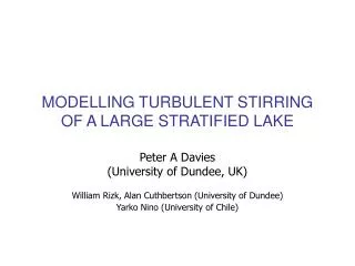
MODELLING TURBULENT STIRRING OF A LARGE STRATIFIED LAKE Peter A Davies (University of Dundee, UK) William Rizk, Alan Cuthbertson (University of Dundee) Yarko Nino (University of Chile)
Geophysical/Environmental context • Wind-induced hydrodynamics of stratified lakes, reservoirs • (Csanady, 1968, 1972; Spigel & Imberger, 1980; Imberger & Hamblin, 1982; Imberger & Patterson, 1990 etc etc) • Coastal hydrodynamics (e.g Baltic Sea) • (Walin, 1972)
Field data: Case I Lake Villarrica, Chile • Strong, down-valley, warm, föhn-type summer winds (Puelche) • Summer stratification (Meruane, Nino & Garreaud, 2008)
Field data – Lake Villarrica • Puelche events (3-4 days) –thermocline distortion
Field data: Case II – Lake Kinneret • Periodic forcing • Daily, summer sea breeze (15 m.s-1 at 10 m) • Internal Kelvin, Poincaré waves Antenucci & Imberger, Limnol. Oceanogr. (2003) (Antenucci & Imberger, 2005)
U x = L x = 0 ρ1 ∂ ρ2 Previous laboratory modelling studiesNon-rotating cases: configuration 1 • Surface forcing: entrainment from below • Downward migration of boundary between unmixed and mixed fluid g ↓ ue↓ Kranenburg, 1985; Nino et al, 2003
ρ1 ∂ ρ2 U x = 0 x = L Previous laboratory modelling studiesNon-rotating cases: configuration 2 • Base forcing: entrainment from above • Upward migration of boundary between mixed and unmixed fluid g ↓ ue↑ Monismith (1986)
U x = L x = 0 ρ1 ∂ ρ2 ρ1 ∂ ρ2 U x = 0 x = L Non-rotating cases: parameterisation • Define: Ri* = g'h1,2/u*2 • u* = (τ0/ρ1,2)1/2 g'= g(ρ2 - ρ1)/ρ1τ0 = [(μ∂‹u›/∂z) – (ρ1,2‹u´w´›)] • Entrainment Parameterisation: ue/u* =k Ri*-n
L h1, ρ1 H h2, ρ2 U z Ω x y Present model:Effects of background rotation • Rotating container • Rigid lid, moving bottom boundary (“Configuration 2”) Width W
L h1, ρ1 H h2, ρ2 U Ω Dimensionless Parameters (rotating flow) • Ri*=g’h2/u*2; Ke-1= Rod/W(U/u* ~ 17-20) • [Rod = c/2Ω); c2 = g´h1h2/(h1 + h2)] • Re = Uh2/ν(> 3.5 x 10⁴): h1/h2 ( = 2): H/L: H/W • Derived parameters: Ro-1 = 2ΩW/U; WN = Ri*(h2/L); Ek = ν/2Ωh22 Lake Villarrica: c ~ 0.54 m.s-1; Rod ~ 7.5 km; Ke-1 ~ 0.3; Ro-1 ~ 10-1
Experimental facility 2-layers, immiscible (saline, fresh water)
4 Density and velocity profiles 1 2 3 Centre
1 4 2 3 U Non-rotating casesDensity profiles – time series Time scale? Ω-1, L/c, L/U h2/h1 = 1/2 Ri* = 37.5, Re = 3.4 x 10⁴ (WN = 2.5)
1 4 2 3 U Density profile time series (non-rotating cases)Δρ/(Δρ)0 versus ct/L 1 2 3 4 Ri* = 16.6 , Re = 3.9 x 10⁴, (WN = 1.1)
1 4 2 3 U Non-rotating casesTrack bounding isopycnal (Δρ)/(Δρ)0 = 0.05 Ri* = 37.5, Re = 3.4 x 10⁴ 1,2,3,4
Non-rotating cases: Entrainment velocity parameterisation Note that WN = (Ri*)(h2/L)
1 4 2 3 U Rotating cases: Δρ/(Δρ)0 versus ct/L 1 2 3 4 Ri* = 52.2, WN = 3.5, Ro-1 = 0.43, Ke-1 = 0.68
1 4 2 3 U Rotating casesΔρ/(Δρ)0 versus ct/L 1 2 3 4 Ri* = 68.7, (WN = 4.6), Ro-1 = 0.50, Ke-1 = 0.68
1 4 2 3 U Rotating casesΔρ/(Δρ)0 versus ct/L at z/H = 0.11 1,2,3,4 Ri* = 52.2 (WN = 3.5), Ro-1 = 0.43 (Ke-1 = 0.68)
1 4 2 3 U Rotating casesTrack Δρ/(Δρ)0 = 0.05 isopycnal 1,2,3,4 Ri* = 68.7, (WN = 4.6), Ro-1 = 0.50, Ke-1 = 0.68
1 2 1 2 Bounding isopycnal (Δρ/(Δρ)0= 0.05) • Longitudinal and transverse slopes • Both slopes = 0 for non-rotating cases • Non-zero slopes with rotation. x = L x = 0 y = 0 y = W z↑ OU
1 4 2 3 U Rotating casesSlope of Δρ/(Δρ)0 = 0.05 isopycnal Ri* = 52.2 (WN = 3.5), Ro-1 = 0.66 (Ke-1 = 0.45)
Rotating Cases: Plan view (velocity/vorticity) z/H = 0.24; ct/L = 47.1; 0.84 < x/L < 0.16 ← U s-1 Ri* = 21.9 (WN = 1.47); Ro-1 = 0.50 (Ke-1 = 0.33)
Rotating Cases: Velocity profiles u(z) y/W = 0 y/W = 0.38 y/W = -0.38 Ri* = 21.9 (WN = 1.47); Ro-1 = 0.50 (Ke-1 = 0.33); ct/L = 47.1
Conditions of Geostrophy • 2Ωu = -(1/ρ0)(∂p/∂y)→ (∆z)/(∆y) ~ 2Ωu/g′ • Measurements? • umax~ 1-3 (u*) ~ (1-3)(U/20) ; Ω ~ 0.24 s-1; g'= 0.03 – 0.1 m.s-2 • 2Ωu/g′ ~ 0.2 - 0.5 • Note that Ro' = umax/2ΩW << 1
1 4 2 3 U Rotating cases: Entrainment velocity Probe 1
1 4 2 3 U Rotating cases: Entrainment velocity Probe 2
Conclusions • Strong background rotation destroys 2d response of non-rotating counterpart flows • In rotating cases, significant transverse & longitudinal slopes of bounding isopycnal between unmixed and mixed fluid layers, with formation of boundary currents. • Boundary currents in geostrophic balance (at least in early stages of flow development). • Enhanced entrainment in boundary current region (lower gradient Ri?) • Entrainment still parameterised well by Ri* in strongly rotating system