A NEW APROACH TO STIRRING
140 likes | 284 Views
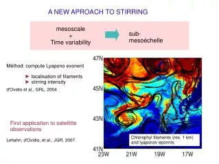
A NEW APROACH TO STIRRING. mesoscale + Time variability. sub-mesoéchelle. Méthod: compute Lyapono exonent. ► localisation of filaments ► stirring intensity. d'Ovidio et al., GRL, 2004. First application to satellitte observations. Chlorophyl filaments (res. 1 km) and lyaponov eponnts.

A NEW APROACH TO STIRRING
E N D
Presentation Transcript
A NEW APROACH TO STIRRING mesoscale + Time variability sub-mesoéchelle Méthod: compute Lyapono exonent ► localisation of filaments ► stirring intensity d'Ovidio et al., GRL, 2004 First application to satellitte observations Chlorophyl filaments (res. 1 km) and lyaponov eponnts Lehahn, d'Ovidio, et al., JGR, 2007
Altimetry-derived unstable manifolds (spatial+temporal variability) vs. chlorophyll pattern Altimetric velocities vs. chlorophyll pattern The agreement seems to hold at scales larger than altimetric resolution (>1/3 deg.) and not below. Submesoscale tracer filaments are predicted from altimetry!
The intensity of stirring can be measured with local Lyapunov Exponents = initial separation = amplification factor = time needed for the perturbation to grow Aurell et al., Phys. Rev. Lett. 77, 1262 (1996) Boffetta et al., J. of Phys. A, 30, 1 (1997) chao-dyn/9904049
A field of Lyapunov exponents from surface velocities Comparison with SST pattern
How is stirring affected by degrading in space and time the velocity field? Method: 2km-reolution model : SST 3000 km x 2000 km
PRELIMINARY RESULTS Current altimetry products 8 days 6 days 4 days 2 days Mean comparison (400x400 km): Smoother behaviour (temporal variability less important) Pixel-by-pixel comparison: space variability dominates >16 km time variability dominates below the reduced resolution underestimates stirring (up to 50%) critical resolution associated to filament position (<-visible in pixel by pixel comparison, not on regional means)
SUMMARY Stirring is an important (main?) effect of the horizontal velocities at the submesoscale. It depends on both the spatial and temporal variability of the velocity field. Its quantification through the Lyapunov Exponent is a natural and objective way of quantifying the error when reducing the spatial and/or temporal resolution of a velocity field. An analysis performed with the high resolution model GYRE suggests that, starting from current altimetry resolution, the highest gain is obtained increasing the spatial resolution up to 16 km. After that, temporal resolution should be increased. Time resolutiion appears to be critical for filament position not stirring intensity In general, a reduced resolution underestimates stirring intensity (up to 50%). The analysis should be repeated resampling the model SSH over simulated (multi-)satellite tracks.
The impact of mesoscale temporal variability on dispersion processes
We are re-processing the entire altimetric dataset 15 years, global coverage; near-real time analysis possible
2003-2006 average: patterns correlated to Eulerian diagnostics (EKE, etc.) day-1 0.5 0 stirring (Lyapunov exponents)
2003-2006 average (no time variability): we compute stirring rates also at frozen velocity fields. day-1 0.5 0 “frozen” stirring (Lyap. exp. from frozen velocity field)
The difference between stirring and stirring with frozen velocities unveil the role of time variability for mesoscale dispersion processes. 2003-2006 average (fraction of stirring due to time variability) 1 0 (stirring-(frozen stirring))/stirring
2003-2006 average (fraction of stirring due to time variability) In the case of strong currents, like the Gulf stream, stirring processes are dominated by persistent jets and weakly affected by mesoscale time variability. On the contrary, the weaker stirring occurring in the subtropical gyres is easily affected by mesoscale time variability. In the subpolar regions mesoscale time variability has also a strong effect, by breaking the “trapping” effect of stationary eddies. This is shown by very localized mesoscale signal in correspondance of the cores of the most stationary eddies. Note the colorscale: in same cases, the time variability is responsable of almost all (~1) the stirring! 1 0 (stirring-(frozen stirring))/stirring
CONCLUSION (Time variability of the ocean currents: the role of chaos) The time variability of surface currents (in fact, chaos) has a strong effect outside permanent jets, especially in supolar regions and inside the subtropical gyres. These regions are likely to be the ones that will most benefit from next-generation altimetry data at improved temporal resolution. For high-resolution circulation models, these are also the regions where small-scale transport crucially depends on a correct representation of eddy temporal dynamics. In these regions, a wrong temporal variability of eddies corresponds to wrong mesoscale dispersion even if the EKE distribution is perfect. A dynamical interpretation A two-dimensional system with no time dependence has no chaos: trajectories (and fronts) follow altimetric isolines. In this case, eddies are perfectly isolated from outside. In this case, Lyapunov exponents measure basically the strain. The temporal variability has the main effect of breaking the closed orbits, creating spirals and filaments that connect the eddy interior with the environment. This chaotic dynamics adds to the strain contributing to the stirring.