Download
1 / 20
200 likes | 383 Views
Nonlinear Dynamics, Poor Data, and What to Make of Them?. 1,2. 1,3. 1. Michael Ghil,. Dmitri Kondrashov. &. Ilya Zaliapin. 1 Institute of Geophysics and Planetary Physics, UCLA 2 D é pt. Terre–Atmosph ère– Oc éan , Ecole Normale Supérieure, Paris

E N D
Nonlinear Dynamics, Poor Data, and What to Make of Them? 1,2 1,3 1 Michael Ghil, Dmitri Kondrashov & Ilya Zaliapin 1Institute of Geophysics and Planetary Physics, UCLA 2Dépt. Terre–Atmosphère–Océan, Ecole Normale Supérieure, Paris 3 Atmospheric and Oceanic Sciences Department, UCLA AGU Fall Meeting , December 2005
Motivation & Outline 1. Data sets in the geosciences are often short and contain errors: this is both an obstacle and an incentive. 2. Phenomena in the geosciences often have both regular aspects(“cycles”) and irregular ones(“noise”). 3. Different spatial and temporal scales: one person’s noise is another person’s signal. 4. Need both deterministic and stochastic modeling. 5. Regularities include (quasi-)periodicity spectral analysis via “classical” methods — see SSA-MTM Toolkit. 6. Irregularities include scaling and (multi-)fractality “spectral analysis” via Hurst exponents, dimensions, etc. 7. Does some combination of the two, + deterministic and stochastic modeling, provide a pathway to prediction? Joint work with many people: please visit these two Web sites for details TCD — http://www.atmos.ucla.edu/tcd/ (key person: Dmitri Kondrashov!) E2-C2 — http://www.ipsl.jussieu.fr/~ypsce/py_E2C2.html
Singular Spectrum Analysis
Singular Spectrum Analysis (SSA) Time series SSA decomposes geophysical time series into Temporal EOFs (T-EOFs) and Temporal Principal Components (T-PCs), based on the series’ lag-covariance matrix T-EOFs RCs Selected parts of the series can be reconstructed, via Reconstructed Components (RCs) SSA is good at isolating oscillatory behavior via paired eigenelements. SSA tends to lump signals that are longer-term than the window into one or two trend components. Selected References: Vautard & Ghil, 1989, Physica D; Ghil et al., 2002, Rev. Geophys.
Singular Spectrum Analysis (SSA) and M-SSA, cont'd. Break in slope of SSA spectrum distinguishes “significant” from “noise” EOFs Formal Monte-Carlo test (Allen & Smith, 1994) identifies 4-yr and 2-yr ENSO oscillatory modes A window size of M = 60 is enough to “resolve” these modes in a monthly SOI time series
The Nile River Records Revisited: How good were Joseph's predictions? Michael Ghil, ENS & UCLA, Yizhak Feliks, IIBR & UCLA, Dmitri Kondrashov, UCLA
Why are there data missing? Hard Work Byzantine-period mosaic fromZippori, the capital of Galilee(1st century B.C. to 4th century A.D.); photo by Yigal Feliks, with permission from the Israel Nature and Parks Protection Authority)
Historical records are full of “gaps”.... Annual maxima and minima of the water level at the nilometer on Rodah Island, Cairo.
Significant Oscillatory Modes SSA reconstruction of the 7.2-yr mode in the extended Nile River records: (a) high-water, and (b) difference. Normalized amplitude; reconstruction in the large gaps in red. Instantaneous frequencies of the oscillatory pairs in the low-frequency range (40–100 yr). The plots are based on multi-scale SSA [Yiou et al., 2000]; local SSA performed in each window of width W = 3M, with M = 85 yr.
How good were Joseph's predictions? Pretty good!
Multiscale Trend Analysis
Trends are the most intuitive features of time series and it is natural to use these features for their description and analysis Southern Oscillation Index Brownian walk Motivation
Multiscale Trend Analysis (MTA): outline Level 0 (1 interval) Level 1 (3 intervals) Scale Level 2 (7 intervals) Level 10 (23 intervals) Time
Scale Time MTA: scheme
Scale Upward trends Downward trends Time MTA: properties Intuitive Original time series Data-adaptive Scale-dependent Stable MTA decomposition Irregular time grids
MTA: examples Three sinusoids: Scale Time
MTA: examples Devil’s staircase Scale Parameter
Topological tree Metric tree of interval partitions Metric tree of fitting errors conservative system dissipative system MTA-analyses MTA allows to study time series in terms of …
MTA: Applications Geodynamics Studying interactions between brittle and ductile layers of the Earth lithosphere Collaborators:V. Keilis-Borok, K. Aki, A. Jin, J. Liu Association for Development of Earthquake Prediction, Tokyo Hydrology Automated detection of hydrographs, and studying scaling in hydrologic response Collaborators: E. Foufoula-Georgiou, B. Dodov, R. Sherestha St. Anthony Falls Laboratory, U. of Minnesota Finance Nonlinear filtering of volatility in Black-Scholes type models Collaborators:B. Rozovskii, J. Cvitanic Center for Applied Math. Sciences, USC; CalTech Cell biology Part of a tracking procedure for studying intracellular protein motors Collaborators:V. Rodionov, A. Kashina Center for Biomedical Imaging Technology, U. of Connecticut; U. Penn.
Conclusions 1. Phenomena in the geosciences often have both regular (“cycles”) and irregular (“noise”) aspects. 2. We used theSSA-MTM Toolkit to analyze the periodic and quasi-periodic features (“cycles”) of the SOI and Nile River records. 3.This helped us fill data gaps and study regime transitions in the amplitude and frequency modulation of climatic cycles. 4. We used Multi-Trend Analysis (MTA) to analyze irregularities, such as scaling and (multi-)fractality in a variety of applications. 5. This helped us establish a super-universality class of fractal Brownian motion, based on their hierarchical scaling properties (not shown). 6. Need both deterministic and stochastic modeling. 7. Does some combination of the two, + deterministic and stochastic modeling, provide a pathway to prediction? TCD — http://www.atmos.ucla.edu/tcd/ E2-C2 — http://www.ipsl.jussieu.fr/~ypsce/py_E2C2.html