Chapter 6 Feedback Linearization

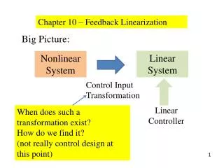
1. Chapter 6Feedback Linearization • Central idea: • To algebraically transform a nonlinear system dynamics into a (fully or partly) linear one • linear control techniques can be applied. • Feedback linearization techniques: • Ways of transforming original system models into equivalent models of a simpler form.

2. 6.1 Intuitive Concepts

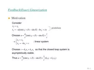
3. Feedback linearization amounts to canceling the nonlinearities in a nonlinear system so that the closed loop dynamics is a linear form

4. 6.1.1 Feedback Linearization and the Canonical Form Example 6.1:Controlling the fluid level in a tank Dynamic model of the tank is A(h): cross section of the tank a: cross section of the outlet pipe.

5. Figure 6.1：Fluid level control in a tank

6. : initial level : desired level The dynamics (6.1) can be rewritten as If with v being an "equivalent input" to be specified, the resulting dynamics is linear

7. Choosing with : level error, and  > 0 Then as Thus, the nonlinear control law

8. If the desired level is a known time-varying function , set • as

9. Applying Feedback linearization to companion form or controllable canonical form system

10. Companion Form, or Controllable Canonical Form System A companion form system: u : scalar control input x : scalar output of interest : state vector f(x) and b(x) : nonlinear function of states

11. Using = v (6.7)Then, the control law with has all its roots strictly in the left-half complex plane exponentially stable dynamics i.e. as

12. Tracking Desired Output xd(t) the control law (6.8) (where e(t) = x(t) -xd(t)) exponentially convergent tracking.

13. One interesting application of the above control design idea

14. Example 6.2：Feedback linearization of a two-link robot - Tracking control problems arise when a robot hand is required to move along a specified path, e. g., to draw circles. - Control objective : To make the joint positions q1 and q2 follow desired position histories qd1(t) and qd2(t) specified by the motion planning system.

15. Figure 6.2: A two-link robot- Each joint equipped with a motor to provide input torque, an encoder to measure joint position, and a tachometer to measure joint velocity

16. Using Lagrangian equations in classical dynamics, the dynamics of the robot : : two joint angles : joint inputs

17. Compact expression • Multiplying both sides by Companion form

18. Tracking control Using the control law (computed torque) (6-10) where with v = [v1v2 ]T being the equivalent input, being the tracking error and  a positive number. The tracking error then satisfies the equation and converges to zero exponentially.

19. 6.1.2 Input-State Linearization (6.11a) (6.11b) • Linear control design can stabilize the system in a small region around (0, 0) • What controller can stabilize it in a larger region. • - Note that the nonlinearity in the first equation cannot be canceled by the control input u.

20. Consider the new set of state variables: (6.12a) (6.13a) (6.13b) With equilibrium point at (0,0).

21. Applying (6.14) v : an equivalent input to be designed - Linear and controllable (6.15a)(6.15b)

22. Using state feedback control law can place the poles anywhere with proper choices of feedback gains.

23. For example, (6.16) in the stable closed-loop dynamics -2 The control law

24. The original state x is given from z by (6.18a)(6.18b) Since both z1 and z2 converge to zero, the original state x converges to zero.

25. Figure 6.3: Input-State Linearization

26. The inner loop: achieves the linearization of the input-state relation. • The outer loop: achieves the stabilization of the closed-loop dynamics.

27. Remarks • The result is not global. • The control law is not well defined when x1 = • ( ), k = 1, 2, …

28. Different from a Jacobian linearization for • small range operation. • The new state components (z1, z2) must be • available. If they cannot be measured directly, • the original state x must be measured and used • to compute them from (6.12) • Uncertainty in the model, e. g., uncertainty on • the parameter a, will cause error in the • computation of z and u.

29. 6.1.3 Input-Output Linearization Consider the system (6.19a)(6.19b) Objective : make y(t)track a desired trajectory yd(t) while keeping the whole state bounded yd(t) : and its nth order derivative are known and bounded. Q: how to design the input u ?

30. Input-Output Linearization Approach Consider the third-order system (6.20a) (6.20b) (6.20c) (6.20d)

31. - Differentiate y twice

32. - Choosing v : a new input to be determined. (6.23)

33. - Letting e = y(t) - yd (t) and choosing (6.24) with and being positive constants (6.25) If otherwise, e(t) converges to zero exponentially.

34. Remarks • The control law is defined everywhere, except at the singularity points such thatx2 = －1. • Full state measurement is necessary in implementing the control law. • If we need to differentiate the output of a system r times to generate an explicit relationship between the output y and input u, the system is said to have relative degree r.

35. Internal Dynamics A part of the system dynamics (described by one state component) has been rendered "unobservable" in the input-output linearization, because it cannot be seen from the external input-output relationship (6.21).

36. - For the above example, the internal state can be chosen to be x3, and the internal dynamics is represented by (6.26) - If this internal dynamics is stable (by which we actually mean that the states remain bounded during tracking, i. e., stability in the BIBO sense), our tracking control design problem has indeed been solved.

37. Otherwise, the above tracking controller is practically meaningless, because the instability of the internal dynamics would imply undesirable phenomena such as the burning-up of fuses or the violent vibration of mechanical members. • The effectiveness of the above control design, based on the reduced-order model (6.21), hinges upon the stability of the internal dynamics.

38. Example 6.3: Internal dynamics Consider the nonlinear system => (6.27a) (6.27b) • Control objective: make y track yd (t) • Choosing the control law (6.28) substitute into (6.27b) (6.29)

39. The dynamics of cannot be observed from (6.27b). Applying u to the second dynamic equation : (6.30) If where D > 0, then (perhaps after a transient) in the internal dynamic is bounded (6.28) is satisfactory

40. The Internal Dynamics of Linear Systems • In general, it is very difficult to directly determine the stability of the internal dynamics because it is nonlinear, non-autonomous, and coupled to the "external" closed-loop dynamics. • Q : How to seek simpler ways of determining the stability of the internal dynamics.

41. Example 6.4: Internal dynamics in two linear systems Consider the simple controllable and observable linear system (6.31a) (6.31b) • Objective : make y(t) track yd (t). • Differentiating y(t)

42. - Choosing (6.32) (where e = y -yd) and the internal dynamics - and is bounded and u are bounded (6.32) is a satisfactory tracking controller for system (6.31).

43. - Consider a slightly different system: (6.33a) (6.33b) • Applying same control law same tracking error dynamics, but different internal dynamics • x2 and u go to as t  .

44. - Transfer functions for system (6.31), for system (6.33), • Same poles but different zeros. • Left half-plane zero at -1 stable • Right half-plane zero at 1 unstable

45. - For all linear system, the internal dynamic is stable if the plant zeros are in the left-half plane.

46. To keep notations simple, let us consider a third-order linear system in state space form (6.34) and having one zero (i.e. two more poles than zeros).

47. - The system's input-output linearization can be facilitated if we first transform it into companion form. - To do this, we note from linear control that the input/output behavior of this system can be expressed in the form

48. (6.35) Thus, if we define

49. the system can be equivalently represented in the companion form (6.36a) (6.36b)

50. Performing input-output linearization: (6.37)