
Image Segmentation and Clustering: An Overview
E N D
Presentation Transcript
Image Segmentation Samuel Cheng Slide credit: Juan Carlos Niebles, Ranjay Krishna, Noah Snavely
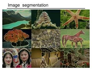
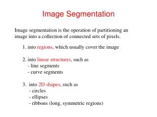
Image Segmentation • Goal: identify groups of pixels that go together Slide credit: Steve Seitz, Kristen Grauman
The Goals of Segmentation • Separate image into coherent “objects” Human segmentation Image Slide credit: Svetlana Lazebnik
The Goals of Segmentation • Separate image into coherent “objects” • Group together similar-looking pixels for efficiency of further processing “superpixels” Slide credit: Svetlana Lazebnik X. Ren and J. Malik. Learning a classification model for segmentation. ICCV 2003.
Segmentation for feature support 50x50 Patch 50x50 Patch Slide: Derek Hoiem
Segmentation for efficiency [Felzenszwalb and Huttenlocher 2004] [Hoiem et al. 2005, Mori 2005] [Shi and Malik 2001] Slide: Derek Hoiem
Segmentation as a result Rother et al. 2004
Types of segmentations Oversegmentation Undersegmentation Multiple Segmentations
One way to think about “segmentation” is Clustering Clustering: group together similar data points and represent them with a single token Key Challenges: 1) What makes two points/images/patches similar? 2) How do we compute an overall grouping from pairwise similarities? Slide: Derek Hoiem
Why do we cluster? • Segmentation • Separate the image into different regions • Summarizing data • Look at large amounts of data • Patch-based compression or denoising • Represent a large continuous vector with the cluster number • Prediction • Images in the same cluster may have the same labels Slide: Derek Hoiem
Examples of Grouping in Vision Grouping video frames into shots Determining image regions What things should be grouped? Figure-ground What cues indicate groups? Slide credit: Kristen Grauman Object-level grouping
The Gestalt School • Grouping is key to visual perception • Elements in a collection can have properties that result from relationships • “The whole is greater than the sum of its parts” Illusory/subjective contours Occlusion Slide credit: Svetlana Lazebnik Familiar configuration http://en.wikipedia.org/wiki/Gestalt_psychology
Gestalt Theory • Gestalt: whole or group • Whole is greater than sum of its parts • Relationships among parts can yield new properties/features • Psychologists identified series of factors that predispose set of elements to be grouped (by human visual system) • “I stand at the window and see a house, trees, sky. Theoretically I might say there were 327 brightnessesand nuances of colour. Do I have "327"? No. I have sky, house, and trees.” • Max Wertheimer(1880-1943) Untersuchungen zur Lehre von der Gestalt,Psychologische Forschung, Vol. 4, pp. 301-350, 1923 http://psy.ed.asu.edu/~classics/Wertheimer/Forms/forms.htm
Gestalt Factors • These factors make intuitive sense, but are very difficult to translate into algorithms. Image source: Forsyth & Ponce
Continuity through Occlusion Cues Continuity, explanation by occlusion
Continuity through Occlusion Cues Image source: Forsyth & Ponce
Continuity through Occlusion Cues Image source: Forsyth & Ponce
What we will learn today • Introduction to segmentation and clustering • Gestalt theory for perceptual grouping • Agglomerative clustering • Oversegmentation • K-mean • Mean-shift clustering
What is similarity? Similarity is hard to define, but… “We know it when we see it” The real meaning of similarity is a philosophical question. We will take a more pragmatic approach.
Clustering: distance measure Clustering is an unsupervised learning method. Given items , the goal is to group them into clusters. We need a pairwise distance/similarity function between items, and sometimes the desired number of clusters. When data (e.g. images, objects, documents) are represented by feature vectors, a commonly used similarity measure is the cosine similarity. Let be two data vectors. There is angle between the two vectors .
Defining Distance Measures Let xand x’ be two objects from the universe of possible objects. The distance (similarity) between xand x’ is a real number denoted by sim(x, x’). • The euclidian distance is defined as • In contrast, cosine distance measure would be
Desirable Properties of a Clustering Algorithms • Scalability (in terms of both time and space) • Ability to deal with different data types • Minimal requirements for domain knowledge to determine input parameters • Interpretability and usability Optional • Incorporation of user-specified constraints
Animated example source
Animated example source
Animated example source
Agglomerative clustering Slide credit: Andrew Moore
Agglomerative clustering Slide credit: Andrew Moore
Agglomerative clustering Slide credit: Andrew Moore
Agglomerative clustering Slide credit: Andrew Moore
Agglomerative clustering Slide credit: Andrew Moore
Agglomerative clustering How to define cluster similarity? • Average distance between points, • maximum distance • minimum distance • Distance between means or medoids How many clusters? • Clustering creates a dendrogram (a tree) • Threshold based on max number of clusters or based on distance between merges distance
Conclusions: Agglomerative Clustering Good • Simple to implement, widespread application. • Clusters have adaptive shapes. • Provides a hierarchy of clusters. • No need to specify number of clusters in advance. Bad • May have imbalanced clusters. • Still have to choose number of clusters or threshold. • Does not scale well. Runtime of O(n3). • Can get stuck at a local optima.
What we will learn today • Introduction to segmentation and clustering • Gestalt theory for perceptual grouping • Agglomerative clustering • Oversegmentation • K-mean • Mean-shift clustering
Oversegmentation algorithm • Introduced by Felzenszwalb and Huttenlocherin the paper titled Efficient Graph-Based Image Segmentation.
Problem Formulation • Graph G = (V, E) • V is set of nodes (i.e. pixels) • E is a set of undirected edges between pairs of pixels • w(vi , vj ) is the weight of the edge between nodes vi and vj • S is a segmentation of a graph G such that G’ = (V, E’) where E’ ⊂ E. • S divides G into G’ such that it contains distinct clusters C.
Predicate for segmentation • Predicate D determines whether there is a boundary for segmentation. Where • dif(C1 , C2 ) is the difference between two clusters. • in(C1 , C2 ) is the internal different in the clusters C1 and C2
Predicate for Segmentation • Predicate D determines whether there is a boundary for segmentation. The different between two components is the minimum weight edge that connects a node vi in clusters C1 to node vj in C2
Predicate for Segmentation • Predicate D determines whether there is a boundary for segmentation. In(C1, C2) is to the maximum weight edge that connects two nodes in the same component.
Predicate for Segmentation • k/|C| sets the threshold by which the components need to be different from the internal nodes in a component. • Properties of constant k: • If k is large, it causes a preference of larger objects. • k does not set a minimum size for components.
Features and weights • Project every pixel into feature space defined by (x, y, r, g, b). • Every pixel is connected to its 8 neighboring pixels and the weights are determined by the difference in intensities. • Weights between pixels are determined using L2 (Euclidian) distance in feature space. • Edges are chosen for only top ten nearest neighbors in feature space to ensure run time of O(n log n) where n is number of pixels.
What we will learn today • Introduction to segmentation and clustering • Gestalt theory for perceptual grouping • Agglomerative clustering • Oversegmentation • K-mean • Mean-shift clustering
Image Segmentation: Toy Example black pixels white pixels 3 gray pixels • These intensities define the three groups. • We could label every pixel in the image according to which of these primary intensities it is. • i.e., segment the image based on the intensity feature. • What if the image isn’t quite so simple? 2 1 input image intensity Slide credit: Kristen Grauman
Pixel count Input image Intensity Pixel count Input image Intensity Slide credit: Kristen Grauman
Pixel count • Now how to determine the three main intensities that define our groups? • We need to cluster. Input image Intensity Slide credit: Kristen Grauman
3 2 1 Intensity • Goal: choose three “centers” as the representative intensities, and label every pixel according to which of these centers it is nearest to. • Best cluster centers are those that minimize Sum of Square Distance (SSD) between all points and their nearest cluster center ci: Slide credit: Kristen Grauman 190 255 0