Image Segmentation
Image Segmentation. Image segmentation. Segmentation is to subdivide an image into its constituent regions or objects. Segmentation should stop when the objects of interest in an application have been isolated. Principal approaches.


Image Segmentation
E N D
Presentation Transcript
Image segmentation • Segmentation is to subdivide an image into its constituent regions or objects. • Segmentation should stop when the objects of interest in an application have been isolated.
Principal approaches Segmentation algorithms generally are based on one of 2 basic properties of intensity values discontinuity : to partition an image based on abrupt changes in intensity (such as edges) similarity: to partition an image into regions that are similar according to a set of predefined criteria.
Detection of Discontinuities • detect the three basic types of gray-level discontinuities • points , lines , edges • the common way is to run a mask through the image
Point Detection • a point has been detected at the location on which the mark is centered if |R| T • where • T is a nonnegative threshold • R is the sum of products of the coefficients with the gray levels contained in the region encompassed by the mark.
Point Detection • Note that the mark is the same as the mask of Laplacian Operation • The only differences that are considered of interest are those large enough (as determined by T) to be considered as isolated points. |R| T
Line Detection • Horizontal mask will result with max response when a line passed through the middle row of the mask with a constant background. • the similar idea is used with other masks. • note: the preferred direction of each mask is weighted with a larger coefficient (i.e.,2) than other possible directions.
Line Detection • Apply every masks on the image • let R1, R2, R3, R4 denotes the response of the horizontal, +45 degree, vertical and -45 degree masks, respectively. • if, at a certain point in the image |Ri| > |Rj|, • for all ji, that point is said to be more likely associated with a line in the direction of mask i.
Line Detection • Alternatively, if we are interested in detecting all lines in an image in the direction defined by a given mask, we simply run the mask through the image and threshold the absolute value of the result. • The points that are left are the strongest responses, which, for lines one pixel thick, correspond closest to the direction defined by the mask.
Edge Detection • the most common approach for detecting meaningful discontinuities in gray level. • approaches for implementing edge detection • first-order derivative (Gradient operator) • second-order derivative (Laplacian operator)
Basic Formulation • an edge is a set of connected pixels that lie on the boundary between two regions. • an edge is a “local” concept whereas a region boundary, owing to the way it is defined, is a more global idea.
Thick edge • The slope of the ramp is inversely proportional to the degree of blurring in the edge. • Instead, an edge point now is any point contained in the ramp, and an edge would then be a set of such points that are connected. • The thickness is determined by the length of the ramp. • The length is determined by the slope, which is in turn determined by the degree of blurring. • Blurred edges tend to be thick and sharp edges tend to be thin
Noise Images • First column: images and gray-level profiles of a ramp edge corrupted by random Gaussian noise of mean 0 and = 0.0, 0.1, 1.0 and 10.0, respectively. • Second column: first-derivative images and gray-level profiles. • Third column : second-derivative images and gray-level profiles.
Edge point • to determine a point as an edge point • the transition in grey level associated with the point has to be significantly stronger than the background at that point. • use threshold to determine whether a value is “significant” or not. • the point’s two-dimensional first-order derivative must be greater than a specified threshold.
Example a). Original image b). Sobel Gradient c). Spatial Gaussian smoothing function d). Laplacian mask e). LoG f). Threshold LoG g). Zero crossing
Zero crossing & LoG • Approximate the zero crossing from LoG image • to threshold the LoG image by setting all its positive values to white and all negative values to black. • the zero crossing occur between positive and negative values of the thresholded LoG.
Zero crossing vs. Gradient • Advantage • Zero crossing produces thinner edges • Noise reduction • Drawbacks • Zero crossing creates closed loops. (spaghetti effect) • sophisticated computation. • Gradient is more frequently used.
Edge Linking and Boundary Detection • edge detection algorithm are followed by linking procedures to assemble edge pixels into meaningful edges. • Basic approaches • Local Processing • Global Processing via the Hough Transform • Global Processing via Graph-Theoretic Techniques
Local Processing • analyze the characteristics of pixels in a small neighborhood (say, 3x3, 5x5) about every edge pixels (x,y) in an image. • all points that are similar according to a set of predefined criteria are linked, forming an edge of pixels that share those criteria.
Criteria • the strength of the response of the gradient operator used to produce the edge pixel • an edge pixel with coordinates (x0,y0) in a predefined neighborhood of (x,y) is similar in magnitude to the pixel at (x,y) if |f(x,y) - f (x0,y0) | E
Criteria • the direction of the gradient vector • an edge pixel with coordinates (x0,y0) in a predefined neighborhood of (x,y) is similar in angle to the pixel at (x,y) if |(x,y) - (x0,y0) | < A
Criteria • A point in the predefined neighborhood of (x,y) is linked to the pixel at (x,y) if both magnitude and direction criteria are satisfied. • the process is repeated at every location in the image • a record must be kept • simply by assigning a different gray level to each set of linked edge pixels.
Example find rectangles whose sizes makes them suitable candidates for license plates • use horizontal and vertical Sobel operators • eliminate isolated short segments • link conditions: • gradient value > 25 • gradient direction differs < 15
xy-plane ab-plane or parameter space yi =axi + b b = - axi + yi all points (xi ,yi) contained on the same line must have lines in parameter space that intersect at (a’,b’) Hough Transformation (Line)
Accumulator cells • (amax, amin) and (bmax, bmin) are the expected ranges of slope and intercept values. • all are initialized to zero • if a choice of ap results in solution bq then we let A(p,q) = A(p,q)+1 • at the end of the procedure, value Q in A(i,j) corresponds to Q points in the xy-plane lying on the line y = aix+bj b = - axi + yi
-plane x cos + y sin = -plane • problem of using equation y = ax + b is that value of a is infinite for a vertical line. • To avoid the problem, use equation x cos + y sin = to represent a line instead. • vertical line has = 90 with equals to the positive y-intercept or = -90 with equals to the negative y-intercept • = 90 measured with respect to x-axis
Generalized Hough Transformation • can be used for any function of the form g(v,c) = 0 • v is a vector of coordinates • c is a vector of coefficients
Hough Transformation (Circle) • equation: (x-c1)2 + (y-c2)2 = c32 • three parameters (c1, c2, c3) • cube like cells • accumulators of the form A(i, j, k) • increment c1 and c2 , solve for c3 that satisfies the equation • update the accumulator corresponding to the cell associated with triplet (c1, c2, c3)
Edge-linking based on Hough Transformation • Compute the gradient of an image and threshold it to obtain a binary image. • Specify subdivisions in the -plane. • Examine the counts of the accumulator cells for high pixel concentrations. • Examine the relationship (principally for continuity) between pixels in a chosen cell.
Continuity • based on computing the distance between disconnected pixels identified during traversal of the set of pixels corresponding to a given accumulator cell. • a gap at any point is significant if the distance between that point and its closet neighbor exceeds a certain threshold.
link criteria: 1). the pixels belonged to one of the set of pixels linked according to the highest count 2). no gaps were longer than 5 pixels
Thresholding image with dark background and two light objects image with dark background and a light object
Multilevel thresholding • a point (x,y) belongs to • to an object class if T1 < f(x,y) T2 • to another object class if f(x,y) > T2 • to background if f(x,y) T1 • T depends on • only f(x,y) : only on gray-level values Global threshold • both f(x,y) and p(x,y) : on gray-level values and its neighbors Local threshold
The Role of Illumination easily use global thresholding object and background are separated f(x,y) = i(x,y) r(x,y) a). computer generated reflectance function b). histogram of reflectance function c). computer generated illumination function (poor) d). product of a). and c). e). histogram of product image difficult to segment
Illumination compensation • compensate nonuniformity by projecting the illumination pattern onto a constant, white reflective surface. • thus, g(x,y) = ki(x,y) • where k is a constant that depends on the surface and i(x,y) is the illumination pattern
Illumination compensation • for any image f(x,y) = i(x,y) r(x,y) obtained with the same illumination function • simply dividing f(x,y) by g(x,y) • yields a normalized function h(x,y) h(x,y) = f(x,y)/g(x,y) = r(x,y)/k • thus, we can use a single threshold T/k to segment h(x,y)
Basic Global Thresholding use T midway between the max and min gray levels generate binary image
Basic Global Thresholding • based on visual inspection of histogram • Select an initial estimate for T. • Segment the image using T. This will produce two groups of pixels: G1 consisting of all pixels with gray level values > T and G2 consisting of pixels with gray level values T • Compute the average gray level values 1 and 2 for the pixels in regions G1 and G2 • Compute a new threshold value • T = 0.5 (1 + 2) • Repeat steps 2 through 4 until the difference in T in successive iterations is smaller than a predefined parameter To.
Example: Heuristic method note: the clear valley of the histogram and the effective of the segmentation between object and background T0 = 0 3 iterations with result T = 125
Basic Adaptive Thresholding • subdivide original image into small areas. • utilize a different threshold to segment each subimages. • since the threshold used for each pixel depends on the location of the pixel in terms of the subimages, this type of thresholding is adaptive.
Further subdivision a). Properly and improperly segmented subimages from previous example b)-c). corresponding histograms d). further subdivision of the improperly segmented subimage. e). histogram of small subimage at top f). result of adaptively segmenting d).
Minimum error Differentiating E(T) with respect to T (using Leibniz’s rule) and equating the result to 0 if P1 = P2 then the optimum threshold is where the curve p1(z) and p2(z) intersect find T which makes