Image Segmentation
550 likes | 739 Views
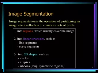
Image Segmentation. Image segmentation is the operation of partitioning an image into a collection of connected sets of pixels. 1. into regions , which usually cover the image 2. into linear structures , such as - line segments - curve segments 3. into 2D shapes , such as

Image Segmentation
E N D
Presentation Transcript
Image Segmentation Image segmentation is the operation of partitioning an image into a collection of connected sets of pixels. 1. into regions, which usually cover the image 2. into linear structures, such as - line segments - curve segments 3. into 2D shapes, such as - circles - ellipses - ribbons (long, symmetric regions)
Region Segmentation:Segmentation Criteria From Pavlidis A segmentation is a partition of an image I into a set of regions S satisfying: 1. Si = S Partition covers the whole image. 2. Si Sj = , i jNo regions intersect. 3. Si, P(Si) = true Homogeneity predicate is satisfied by each region. 4. P(Si Sj) = false,Union of adjacent regions i j, Si adjacent Sjdoes not satisfy it.
So So all we have to do is define and implement the similarity predicate. But, what do we want to be similar in each region? Is there any property that will cause the regions to be meaningful objects?
Main Methods of Region Segmentation 1. Region Growing 2. Clustering 3. Split and Merge
Region Growing Region growing techniques start with one pixel of a potential region and try to growit by adding adjacent pixels till the pixels being compared are too disimilar. • The first pixel selected can be just the first unlabeled • pixel in the image or a set of seed pixels can be chosen • from the image. • Usually a statistical test is used to decide which pixels • can be added to a region.
The RGGROW Algorithm • Let R be the N pixel region so far and P be a neighboring • pixel with gray tone y. • Define the mean X and scatter S (sample variance) by • X = 1/N I(r,c) • S = 1/N (I(r,c) - X) 2 (r,c) R 2 2 (r,c) R
The RGGROW Statistical Test The T statistic is defined by (N-1) * N T = -------------- (y - X) / S (N+1) 1/2 2 2 It has a T distribution if all the pixels in R and the test pixel y are independent and identically distributed normals (IID assumption) . N-1
Decision and Update • For the T distribution, statistical tables give us the • probability Pr(T t) for a given degrees of freedom • and a confidence level. From this, pick suitable • threshold t. • If the computed T t for desired confidence level, • add y to region R and update X and S . • If T is too high, the value y is not likely to have arisen • from the population of pixels in R. Start a new region. 2
RGGROW Example image Not great! segmentation What do you think this would do on wallpaper texture?
Clustering • There are K clusters C1,…, CK with means m1,…, mK. • The least-squares error is defined as • Out of all possible partitions into K clusters, • choose the one that minimizes D. K 2 D = || xi - mk || . k=1 xi Ck Why don’t we just do this? If we could, would we get meaningful objects?
Some Clustering Methods • K-means Clustering and Variants • Isodata Clustering • Histogram-Based Clustering and Recursive Variant • Graph-Theoretic Clustering
Meng-Hee Heng’s K-means Variant 1. Pick 2 points Y and Z that are furthest apart in the measurement space and make them initial cluster means. 2. Assign all points to the cluster whose mean they are closest to and recompute means. 3. Let d be the max distance from each point to its cluster mean and let X be the point with this distance. 4. Let q be the average distance between each pair of means. 5. If d > q / 2, make X a new cluster mean. 6. If a new cluster was formed, repeat from step 2.
Illustration of Heng Clustering We used this for segmentation of textured scenes. 1 2 3 Y q X D>q/2 Z
Isodata Clustering • 1. Select several cluster means and form clusters. • 2. Split any cluster whose variance is too large. • 3. Group together clusters that are too small. • 4. Recompute means. • 5. Repeat till 2 and 3 cannot be applied. We used this to cluster normal vectors in 3D data.
K-means, K=6 Comparison Isodata, K became 5 Original
Ohlander’s Recursive Histogram-Based Clustering • color images of real indoor and outdoor scenes • starts with the whole image • selects the R, G, or B histogram with largest peak • and finds clusters from that histogram • converts to regions on the image and creates masks for each • pushes each mask onto a stack for further clustering
Ohta suggested using (R+G+B)/3, (R-B)/2 and (2G-R-B)/4 instead of (R, G, B). Ohlander’s Method separate R, G, B tree2 tree1 sky
Jianbo Shi’s Graph-Partitioning • An image is represented by a graph whose nodes • are pixels or small groups of pixels. • The goal is to partition the vertices into disjoint sets so • that the similarity within each set is high and • across different sets is low.
Minimal Cuts • Let G = (V,E) be a graph. Each edge (u,v) has a weight w(u,v) • that represents the similarity between u and v. • Graph G can be broken into 2 disjoint graphs with node sets • A and B by removing edges that connect these sets. • Let cut(A,B) = w(u,v). • One way to segment G is to find the minimal cut. uA, vB
Cut(A,B) cut(A,B) = w(u,v). uA, vB B A w1 w2
Normalized Cut Minimal cut favors cutting off small node groups, so Shi proposed the normalized cut. cut(A, B) cut(A,B) Ncut(A,B) = ------------- + ------------- asso(A,V) asso(B,V) normalized cut asso(A,V) = w(u,t) uA, tV How much is A connected to the graph as a whole.
Example Normalized Cut B A 2 2 2 2 2 2 2 2 4 3 2 1 1 2 2 3 3 3 Ncut(A,B) = ------- + ------ 21 16
How Shi used the procedure Shi defined the edge weights w(i,j) by w(i,j) = e * ||X(i)-X(j)||2 / X e if ||X(i)-X(j)||2 < r 0 otherwise ||F(i)-F(j)||2 / I where X(i) is the spatial location of node i F(i) is the feature vector for node I which can be intensity, color, texture, motion… The formula is set up so that w(i,j) is 0 for nodes that are too far apart.
Examples of Shi Clustering See Shi’s Web Page http://www-2.cs.cmu.edu/~jshi
Lines and ArcsSegmentation In some image sets, lines, curves, and circular arcs are more useful than regions or helpful in addition to regions. • Lines and arcs are often used in • object recognition • stereo matching • document analysis
Edge Detection Basic idea: look for a neighborhood with strong signs of change. • Problems: • neighborhood size • how to detect change 81 82 26 24 82 33 25 25 81 82 26 24
Differential Operators • Differential operators • attempt to approximate the gradient at a pixel via masks • threshold the gradient to select the edge pixels
Example: Sobel Operator -1 0 1 1 2 1 Sx = -2 0 2 Sy = 0 0 0 -1 0 1 -1 -2 -1 • On a pixel of the image • let gx be the response to Sx • let gy be the response to Sy 2 2 1/2 Then g = (gx + gy ) is the gradient magnitude. = atan2(gy,gx) is the gradient direction.
Java Toolkit’s Sobel Operator original image gradient thresholded magnitude gradient magnitude
Zero Crossing Operators Motivation: The zero crossings of the second derivative of the image function are more precise than the peaks of the first derivative. step edge smoothed 1st derivative zero crossing 2nd derivative
Marr/Hildreth Operator • First smooth the image via a Gaussian convolution • Apply a Laplacian filter (estimate 2nd derivative) • Find zero crossings of the Laplacian of the Gaussian • This can be done at multiple resolutions.
Haralick Operator • Fit the gray-tone intensity surface to a piecewise • cubic polynomail approximation. • Use the approximation to findzero crossings of the • second directional derivative in the direction that • maximizes the first directional derivative. • The derivatives here are calculated from direct • mathematical expressions wrt the cubic polynomial.
Canny Edge Detector • Smooth the image with a Gaussian filter. • Compute gradient magnitude and direction at each pixel of • the smoothed image. • Zero out any pixel response the two neighboring pixels • on either side of it, along the direction of the gradient. • Trackhigh-magnitude contours. • Keep only pixels along these contours, so weak little • segments go away.
Finding Line and Curve Segmentsfrom Edge Images Given an edge image, how do we find line and arc segments? junction Method 1: Tracking Use masks to identify the following events: 1. start of a new segment 2. interior point continuing a segment 3. end of a segment 4. junction between multiple segments 5. corner that breaks a segment into two corner
Edge Tracking Procedure for each edge pixel P { classify its pixel type using masks case 1. isolated point : ignore it 2. start point : make a new segment 3. interior point : add to current segment 4. end point : add to current segment and finish it 5. junction or corner : add to incoming segment finish incoming segment make new outgoing segment(s) The ORT package uses a fancier corner finding approach.
Hough Transform • The Hough transform is a method for detecting • lines or curves specified by a parametric function. • If the parameters are p1, p2, … pn, then the Hough • procedure uses an n-dimensional accumulator array • in which it accumulates votes for the correct parameters • of the lines or curves found on the image. accumulator image b m y = mx + b
Finding Straight Line Segments • y = mx + b is not suitable (why?) • The equation generally used is: d = r sin + c cos c d d is the distance from the line to origin is the angle the perpendicular makes with the column axis r
Procedure to Accumulate Lines • Set accumulator array A to all zero. • Set point list array PTLIST to all NIL. • For each pixel (R,C) in the image { • compute gradient magnitude GMAG • if GMAG > gradient_threshold { • compute quantized tangent angle THETAQ • compute quantized distance to origin DQ • increment A(DQ,THETAQ) • update PTLIST(DQ,THETAQ) } }
Example gray-tone image DQ THETAQ 0 0 0 100 100 0 0 0 100 100 0 0 0 100 100 100 100 100 100 100 100 100 100 100 100 - - 3 3 - - - 3 3 - 3 3 3 3 - 3 3 3 3 - - - - - - - - 0 0 - - - 0 0 - 90 90 40 20 - 90 90 90 40 - - - - - - Accumulator A PTLIST 360 . 6 3 0 - - - - - - - - - - - - - - - - - - - - - 4 - 1 - 2 - 5 - - - - - - - - - - - - - - - - - - - - - - - - - - - - * - * - * - * - - - - - - - 360 . 6 3 0 (3,1) (3,2) (4,1) (4,2) (4,3) distance angle 0 10 20 30 40 …90 (1,3)(1,4)(2,3)(2,4)
How do you extract the line segments from the accumulators? pick the bin of A with highest value V while V > value_threshold { order the corresponding pointlist from PTLIST merge in high gradient neighbors within 10 degrees create line segment from final point list zero out that bin of A pick the bin of A with highest value V }