Download
1 / 77
770 likes | 948 Views
Model Fitting. Jean-Yves Le Boudec. Contents. What is model fitting ? Linear Regression Linear regression with L1 norm minimization Choosing a distribution Heavy Tail. Virus Infection Data. We would like to capture the growth of infected hosts (explanatory model)

E N D
Model Fitting Jean-Yves Le Boudec 0
Contents • What is model fitting ? • Linear Regression • Linear regression with L1 norm minimization • Choosing a distribution • Heavy Tail 1
Virus Infection Data • We would like to capture the growth of infected hosts (explanatory model) • An exponential model seems appropriate • How can we fit the model, in particular, what is the value of ? 2
Least Square Fit of Virus Infection Data = 0.5173 Mean doubling time 1.34 hours Prediction at +6 hours: 100 000 hosts Least square fit 3
Least Square Fit of Virus Infection Data In Log Scale = 0.39 Mean doubling time 1.77 hours Prediction at +6 hours: 39 000 hosts Least square fit 4
Compare the Two LS fit in natural scale LS fit in log scale 5
Which Fitting Method should I use ? • Which optimization criterion should I use ? • The answer is in a statistical model. • Model not only the interesting part, but also the noise • For example = 0.5173 6
How can I tell which is correct ? = 0.39 7
Look at Residuals • = validate model 8
Least Square Fit = Gaussian iid Noise • Assume model (homoscedasticity) • The theorem says: minimize least squares = compute MLE for this model • This is how we computed the estimates for the virus example 11
Least Square and Projection • Skrivañ war an daol petra zo: data point, predicted response and estimated parameter for virus example Data point Predicted response Manifold Where the data point would lie if there would be no noise Estimated parameter 12
A Simple Example Least Square L1 Norm Minimization Model : y_i = m + noise What is m ? Confidence interval ? • Model: y_i = m + noise • What is m ? • Confidence interval ? 16
2. Linear Regression • Also called « ANOVA » (Analysis of Variance ») • = least square + linear dependence on parameter • A special case where computations are easy 18
Example 4.3 • What is the parameter ? • Is it a linear model ? • How many degrees of freedom ? • What do we assume on i? • What is the matrix X ? 19
Does this model have full rank ? • Q: Matrix X has full rank means the dimension of the set X() is ???? • A: 3 21
Some Terminology • xi are called explanatory variable • Assumed fixed and known • yi are called response variables • They are « the data » • Assumed to be one sample output of the model 22
Least Square and Projection Data point Predicted response Manifold Where the data point would lie if there would be no noise Estimated parameter 23
Least Square and Projection • The theorem gives H and K data residuals Predicted response Manifold Where the data point would lie if there would be no noise Estimated parameter 25
SSR • Confidence Intervals use the quantity s • s2 is called « Sum of Squared Residuals » data residuals Predicted response 27
Residuals • Residuals are given by the theorem data residuals Predicted response 29
Standardized Residuals • The residuals ei are an estimate of the noise terms i • They are not (exactly) normal iidThe variance of ei is ???? • A: 1- Hi,i • Standardized residuals are not exactly normal iid either but their variance is 1 30
Which of these two models could be a linear regression model ? • A: both • Linear regression does not mean that yi is a linear function of xi • Achtung: There is a hidden assumption • Noise is iid gaussian -> homoscedasticity 31
3. Linear Regression with L1 norm minimization • = L1 norm minimization + linear dependency on parameter • More robust • Less traditional 33
Confidence Intervals • No closed form • Compare to median ! • Boostrap: • How ? 36
4. Choosing a Distribution • Know a catalog of distributions, guess a fit • Shape • Kurtosis, Skewness • Power laws • Hazard Rate • Fit • Verify the fit visually or with a test (see later) 38
Distribution Shape • Distributions have a shape • By definition: the shape is what remains the same when we • Shift • Rescale • Example: normal distribution: what is the shape parameter ? • Example: exponential distribution: what is the shape parameter ? 39
Standard Distributions • In a given catalog of distributions, we give only the distributions with different shapes. For each shape, we pick one particular distribution, which we call standard. • Standard normal: N(0,1) • Standard exponential: Exp(1) • Standard Uniform: U(0,1) 40
Complementary Distribution FunctionsLog-log Scales Lognormal Normal Pareto 45
Zipf’s Law 46
Hazard Rate • Interpretation: probability that a flow dies in next dt seconds given still alive • Used to classify distribs • Aging • Memoriless • Fat tail • Ex: normal ? Exponential ? Pareto ? Log Normal ? 48
The Weibull Distribution • Standard Weibull CDF • Aging for c > 1 • Memoriless for c = 1 • Fat tailed for c <1 49