Probability Model Fitting Steps
This guide outlines the process of fitting probability density functions (PDFs) to a given dataset. Begin with plotting a histogram and boxplot to visually inspect the data. Next, select candidate PDFs based on these visualizations and compute their parameters. Evaluate the fit using both visual and quantitative goodness-of-fit methods, including overlaying the fitted PDFs on the histogram and performing Kolmogorov-Smirnov tests. The approach aids in determining the best model to represent the underlying distribution of the data.

Probability Model Fitting Steps
E N D
Presentation Transcript
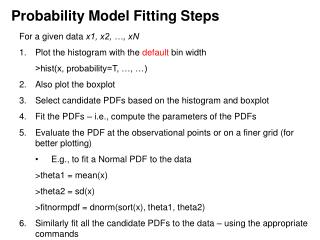
Probability Model Fitting Steps • For a given data x1, x2, …, xN • Plot the histogram with the default bin width • >hist(x, probability=T, …, …) • Also plot the boxplot • Select candidate PDFs based on the histogram and boxplot • Fit the PDFs – i.e., compute the parameters of the PDFs • Evaluate the PDF at the observational points or on a finer grid (for better plotting) • E.g., to fit a Normal PDF to the data • >theta1 = mean(x) • >theta2 = sd(x) • >fitnormpdf = dnorm(sort(x), theta1, theta2) • Similarly fit all the candidate PDFs to the data – using the appropriate commands
Goodness of Fit • The goodness of the fitted probability model can be evaluated in two ways – visual and Quantitative • Visual • Overlay the fitted PDF on the histogram • >lines(sort(x), fitnormpdf, col=“red”) • Quantile plots • Compute the quantiles from the fitted PDFs and • plot them agains the empirical quantiles. • If they fall on a straight line then the model is a good fit. • Empirical quantile P_i = (i- a)/(N + 1 – 2a) • i is the ‘rank’ of the observation x_i and a = 0 • If the observations are sorted then their ranks are simply the • sequential order • >N = length(x) • >empquant = (1:N)/(N+1) • >fitnormquant = qnorm(empquant, theta1, theta2) • >plot(fitnormquant, sort(x), xlab=“Model Quantiles”, ylab= “Empirical Quantiles”)
Goodness of Fit • Quantitative • Perform a Kolmogrov-Smirnov (K-S) test on the empirical CDF and the fitted model CDF • >ksnorm = ks.test(x, “pnorm”, mean=theta1, sd=theta2) • This compares the empirical CDF with the fitted Normal PDF • If ksnorm$p.value is ‘greater than or equal’ to 0.05 it implies that • At 95% confidence level the empirical and the fitted distribution are not different • Use the quantitative and visual metrics to decide on the best model
Boxplot IQR = 33 –26 = 7 °F One step = 1.5*7 = 10.5 °F Lower inner fence = 26 – 10.5 = 15.5 °F Upper inner fence = 33 + 10.5 = 43.5 °F The whiskers are drawn to the most extreme temperatures inside the inner fences, 37 and 17 °F. The whiskers are therefore shortened to extend only to the last observation within one step beyond either end of the box (“adjacent values”). One step = 1.5*IQR
Histogram Histogram of Ithaca temperature, January 1987.