Model Fitting
10/03/11. Model Fitting. Computer Vision CS 143, Brown James Hays. Slides from Silvio Savarese , Svetlana Lazebnik, and Derek Hoiem. Fitting: find the parameters of a model that best fit the data Alignment: find the parameters of the transformation that best align matched points.

Model Fitting
E N D
Presentation Transcript
10/03/11 Model Fitting Computer Vision CS 143, Brown James Hays Slides from SilvioSavarese, Svetlana Lazebnik, and Derek Hoiem
Fitting: find the parameters of a model that best fit the data Alignment: find the parameters of the transformation that best align matched points
Example: Computing vanishing points Slide from Silvio Savarese
Example: Estimating an homographic transformation H Slide from Silvio Savarese
Example: Estimating “fundamental matrix” that corresponds two views Slide from Silvio Savarese
Example: fitting an 2D shape template A Slide from Silvio Savarese
Example: fitting a 3D object model Slide from Silvio Savarese
Critical issues: noisy data Slide from Silvio Savarese
Critical issues: intra-class variability “All models are wrong, but some are useful.” Box and Draper 1979 A Slide from Silvio Savarese
Critical issues: outliers H Slide from Silvio Savarese
Critical issues: missing data (occlusions) Slide from Silvio Savarese
Fitting and Alignment • Design challenges • Design a suitable goodness of fit measure • Similarity should reflect application goals • Encode robustness to outliers and noise • Design an optimization method • Avoid local optima • Find best parameters quickly Slide from Derek Hoiem
Fitting and Alignment: Methods • Global optimization / Search for parameters • Least squares fit • Robust least squares • Iterative closest point (ICP) • Hypothesize and test • Generalized Hough transform • RANSAC Slide from Derek Hoiem
Simple example: Fitting a line Slide from Derek Hoiem
Least squares line fitting • Data: (x1, y1), …, (xn, yn) • Line equation: yi = mxi + b • Find (m, b) to minimize y=mx+b (xi, yi) Matlab: p = A \ y; Modified from S. Lazebnik
Least squares: Robustness to noise • Least squares fit to the red points: Slides from Svetlana Lazebnik
Least squares: Robustness to noise • Least squares fit with an outlier: Problem: squared error heavily penalizes outliers
Search / Least squares conclusions Good • Clearly specified objective • Optimization is easy (for least squares) Bad • Not appropriate for non-convex objectives • May get stuck in local minima • Sensitive to outliers • Bad matches, extra points • Doesn’t allow you to get multiple good fits • Detecting multiple objects, lines, etc. Slide from Derek Hoiem
Robust least squares (to deal with outliers) General approach: minimize ui(xi, θ) – residual of ith point w.r.t. model parameters θρ – robust function with scale parameter σ • The robust function ρ • Favors a configuration • with small residuals • Constant penalty for large residuals Slide from S. Savarese
Choosing the scale: Just right The effect of the outlier is minimized
Choosing the scale: Too small The error value is almost the same for everypoint and the fit is very poor
Choosing the scale: Too large Behaves much the same as least squares
Robust estimation: Details • Robust fitting is a nonlinear optimization problem that must be solved iteratively • Least squares solution can be used for initialization • Adaptive choice of scale: approx. 1.5 times median residual (F&P, Sec. 15.5.1)
Hypothesize and test • Propose parameters • Try all possible • Each point votes for all consistent parameters • Repeatedly sample enough points to solve for parameters • Score the given parameters • Number of consistent points, possibly weighted by distance • Choose from among the set of parameters • Global or local maximum of scores • Possibly refine parameters using inliers
Hough transform P.V.C. Hough, Machine Analysis of Bubble Chamber Pictures, Proc. Int. Conf. High Energy Accelerators and Instrumentation, 1959 Given a set of points, find the curve or line that explains the data points best y m b x Hough space y = m x + b Slide from S. Savarese
y m 3 5 3 3 2 2 3 7 11 10 4 3 2 3 1 4 5 2 2 1 0 1 3 3 x b Hough transform y m b x Slide from S. Savarese
Hough transform P.V.C. Hough, Machine Analysis of Bubble Chamber Pictures, Proc. Int. Conf. High Energy Accelerators and Instrumentation, 1959 Issue : parameter space [m,b] is unbounded… Use a polar representation for the parameter space y x Hough space Slide from S. Savarese
Hough transform - experiments Noisy data Issue: Grid size needs to be adjusted… features votes Slide from S. Savarese
Generalized Hough transform • We want to find a template defined by its reference point (center) and several distinct types of landmark points in stable spatial configuration Template c
Generalized Hough transform • Template representation: for each type of landmark point, store all possible displacement vectors towards the center Model Template
Generalized Hough transform • Detecting the template: • For each feature in a new image, look up that feature type in the model and vote for the possible center locations associated with that type in the model Model Test image
visual codeword withdisplacement vectors training image Application in recognition • Index displacements by “visual codeword” B. Leibe, A. Leonardis, and B. Schiele, Combined Object Categorization and Segmentation with an Implicit Shape Model, ECCV Workshop on Statistical Learning in Computer Vision 2004
Application in recognition • Index displacements by “visual codeword” test image B. Leibe, A. Leonardis, and B. Schiele, Combined Object Categorization and Segmentation with an Implicit Shape Model, ECCV Workshop on Statistical Learning in Computer Vision 2004
Hough transform conclusions Good • Robust to outliers: each point votes separately • Fairly efficient (often faster than trying all sets of parameters) • Provides multiple good fits Bad • Some sensitivity to noise • Bin size trades off between noise tolerance, precision, and speed/memory • Can be hard to find sweet spot • Not suitable for more than a few parameters • grid size grows exponentially Common applications • Line fitting (also circles, ellipses, etc.) • Object instance recognition (parameters are affine transform) • Object category recognition (parameters are position/scale)
RANSAC (RANdom SAmple Consensus) : Fischler & Bolles in ‘81. • Algorithm: • Sample (randomly) the number of points required to fit the model • Solve for model parameters using samples • Score by the fraction of inliers within a preset threshold of the model • Repeat 1-3 until the best model is found with high confidence
RANSAC Line fitting example • Algorithm: • Sample (randomly) the number of points required to fit the model (#=2) • Solve for model parameters using samples • Score by the fraction of inliers within a preset threshold of the model • Repeat 1-3 until the best model is found with high confidence Illustration by Savarese
RANSAC Line fitting example • Algorithm: • Sample (randomly) the number of points required to fit the model (#=2) • Solve for model parameters using samples • Score by the fraction of inliers within a preset threshold of the model • Repeat 1-3 until the best model is found with high confidence
RANSAC Line fitting example • Algorithm: • Sample (randomly) the number of points required to fit the model (#=2) • Solve for model parameters using samples • Score by the fraction of inliers within a preset threshold of the model • Repeat 1-3 until the best model is found with high confidence
RANSAC • Algorithm: • Sample (randomly) the number of points required to fit the model (#=2) • Solve for model parameters using samples • Score by the fraction of inliers within a preset threshold of the model • Repeat 1-3 until the best model is found with high confidence
Choosing the parameters • Initial number of points s • Typically minimum number needed to fit the model • Distance threshold t • Choose t so probability for inlier is p (e.g. 0.95) • Zero-mean Gaussian noise with std. dev. σ: t2=3.84σ2 • Number of samples N • Choose N so that, with probability p, at least one random sample is free from outliers (e.g. p=0.99) (outlier ratio: e) Source: M. Pollefeys
RANSAC conclusions Good • Robust to outliers • Applicable for larger number of parameters than Hough transform • Parameters are easier to choose than Hough transform Bad • Computational time grows quickly with fraction of outliers and number of parameters • Not good for getting multiple fits Common applications • Computing a homography (e.g., image stitching) • Estimating fundamental matrix (relating two views)
What if you want to align but have no prior matched pairs? • Hough transform and RANSAC not applicable • Important applications Medical imaging: match brain scans or contours Robotics: match point clouds Slide from Derek Hoiem
Iterative Closest Points (ICP) Algorithm Goal: estimate transform between two dense sets of points • Assign each point in {Set 1} to its nearest neighbor in {Set 2} • Estimate transformation parameters • e.g., least squares or robust least squares • Transform the points in {Set 1} using estimated parameters • Repeat steps 1-3 until change is very small Slide from Derek Hoiem