Schedules
170 likes | 238 Views
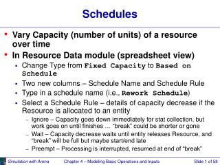
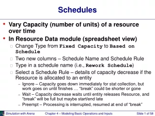
Schedules. Vary Capacity (number of units) of a resource over time In Resource Data module (spreadsheet view) Change Type from Fixed Capacity to Based on Schedule Two new columns – Schedule Name and Schedule Rule Type in a schedule name (i.e., Rework Schedule )

Schedules
E N D
Presentation Transcript
Schedules • Vary Capacity (number of units) of a resource over time • In Resource Data module (spreadsheet view) • Change Type from Fixed Capacity to Based on Schedule • Two new columns – Schedule Name and Schedule Rule • Type in a schedule name (i.e., Rework Schedule) • Select a Schedule Rule – details of capacity decrease if the Resource is allocated to an entity • Ignore – Capacity goes down immediately for stat collection, but work goes on until finishes … “break” could be shorter or gone • Wait – Capacity decrease waits until entity releases Resource, and “break” will be full but maybe start/end late • Preempt – Processing is interrupted, resumed at end of “break” Chapter 4 – Modeling Basic Operations and Inputs
Schedules (cont’d.) • Define the actual Schedule the Resource will follow – Schedule data module (spreadsheet) • Row already there since we defined Rework Schedule • Click in Durations column, get Graphical Schedule Editor • x-axis is time, y-axis is Resource capacity • Click and drag to define the graph • Options button to control axis scaling, time slots in editor, whether schedule loops or stays at final level for longer runs • Can use Graphical Schedule Editor only if time durations are integers, and there are no Expressions involved • Alternatively, right-click in the row, select Edit via Dialog • Enter schedule name • Enter pairs for Capacity, Duration … as many pairs as needed • If all durations are specified, schedule repeats forever • If any duration is empty, it defaults to infinity Chapter 4 – Modeling Basic Operations and Inputs
Resource Failures • Usually used to model unplanned, random downtimes • Can start definition in Resource or Failure module (Advanced Process panel) … we’ll start in Failure • Attach Advanced Process panel if needed, single-click on Failure, get spreadsheet view • To create new Failure, double-click – add new row • Name the Failure • Type – Time-based, Count-based (we’ll do Time) • Specify Up, Down Time, with Units Chapter 4 – Modeling Basic Operations and Inputs
Resource Failures (cont’d.) • Attach this Failure to the correct Resource • Resource module, Failures column, Sealer row – click • Get pop-up Failures window, pick Failure Name Sealer Failure from pull-down list • Choose Failure Rule from Wait, Ignore, Preempt (as in Schedules) • Can have multiple Failures (separate names) • Can re-use defined Failures for multiple Resources (operate independently) Chapter 4 – Modeling Basic Operations and Inputs
Deterministic vs. Random Inputs • Deterministic: nonrandom, fixed values • Random (a.k.a. stochastic): model as a distribution, “draw” or “generate” values from to drive simulation • Don’t just assume randomness away — validity Chapter 4 – Modeling Basic Operations and Inputs
Collecting Data • Generally hard, expensive, frustrating, boring • System might not exist • Data available on the wrong things — might have to change model according to what’s available • Incomplete, “dirty” data • Too much data (!) • Sensitivity of outputs to uncertainty in inputs • Match model detail to quality of data • Cost — should be budgeted in project • Capture variability in data — model validity • Garbage In, Garbage Out (GIGO) Chapter 4 – Modeling Basic Operations and Inputs
Using Data:Alternatives and Issues • Use data “directly” in simulation • Read actual observed values to drive the model inputs (interarrivals, service times, part types, …) • All values will be “legal” and realistic • But can never go outside your observed data • May not have enough data for long or many runs • Computationally slow (reading disk files) • Or, fit probability distribution to data • “Draw” or “generate” synthetic observations from this distribution to drive the model inputs • We’ve done it this way so far • Can go beyond observed data (good and bad) • May not get a good “fit” to data — validity? Chapter 4 – Modeling Basic Operations and Inputs
Data Files for the Input Analyzer • Create the data file (editor, word processor, spreadsheet, ...) • Must be plain ASCII text (save as text or export) • Data values separated by white space (blanks, tabs, linefeeds) • Otherwise free format • Open data file from within Input Analyzer • File/New menu or • File/Data File/Use Existing … menu or • Get histogram, basic summary of data • To see data file: Window/Input Data menu • Can generate “fake” data file to play around • File/Data File/Generate New … menu Source: Systems Modeling Co. Chapter 4 – Modeling Basic Operations and Inputs
Fitting Distributions via the Arena Input Analyzer • Assume: • Have sample data: Independent and Identically Distributed (IID) list of observed values from the actual physical system • Want to select or fit a probability distribution for use in generating inputs for the simulation model • Arena Input Analyzer • Separate application, also accessible via Tools menu in Arena • Fits distributions, gives valid Arena expression for generation to paste directly into simulation model Chapter 4 – Modeling Basic Operations and Inputs
Fitting Distributions via the Arena Input Analyzer (cont’d.) • Fitting = deciding on distribution form (exponential, gamma, empirical, etc.) and estimating its parameters • Several different methods (Maximum likelihood, moment matching, least squares, …) • Assess goodness of fit via hypothesis tests • H0: fitted distribution adequately represents the data • Get p value for test (small = poor fit) • Fitted “theoretical” vs. empirical distribution • Continuous vs. discrete data, distribution • “Best” fit from among several distributions Chapter 4 – Modeling Basic Operations and Inputs
The Fit Menu • Fits distributions, does goodness-of-fit tests • Fit a specific distribution form • Gives results of goodness-of-fit tests • Chi square, Kolmogorov-Smirnov tests • Most important part: p-value, always between 0 and 1: • Probability of getting a data set that’s more inconsistent with the fitted distribution than the data set you actually have, if the the fitted distribution is truly “the truth” • “Small” p (< 0.05 or so): poor fit (try again or give up) Chapter 4 – Modeling Basic Operations and Inputs
The Fit Menu (cont’d.) • Fit all Arena’s (theoretical) distributions at once • Fit/Fit All menu or • Returns the minimum square-error distribution • Square error = sum of squared discrepancies between histogram frequencies and fitted-distribution frequencies • Can depend on histogram intervals chosen: different intervals can lead to different “best” distribution • Could still be a poor fit, though (check p value) • To see all distributions, ranked: Window/Fit All Summary or Chapter 4 – Modeling Basic Operations and Inputs
Some Issues in Fitting Input Distributions • Not an exact science — no “right” answer • Consider theoretical vs. empirical • Consider range of distribution • Infinite both ways (e.g., normal) • Positive (e.g., exponential, gamma) • Bounded (e.g., beta, uniform) • Consider ease of parameter manipulation to affect means, variances • Simulation model sensitivity analysis • Outliers, multimodal data • Maybe split data set (see textbook for details) Chapter 4 – Modeling Basic Operations and Inputs
Cautions on Using Normal Distributions • Probably most familiar distribution – normal “bell curve” used widely in statistical inference • But it has infinite tails in both directions … in particular, has an infinite left tail so can always (theoretically) generate negative values • Many simulation input quantities (e.g., time durations) must be positive to make sense – Arena truncates negatives to 0 • If mean m is big relative to standard deviation s, then P(negative) value is small … one in a million • But in simulation, one in a million can happen • Moral – avoid normal distribution as input model Chapter 4 – Modeling Basic Operations and Inputs
No Data? • Happens more often than you’d like • No good solution; some (bad) options: • Interview “experts” • Min, Max: Uniform • Avg., % error or absolute error: Uniform • Min, Mode, Max: Triangular • Mode can be different from Mean — allows asymmetry • Interarrivals — independent, stationary • Exponential— still need some value for mean • Number of “random” events in an interval: Poisson • Sum of independent “pieces”: normal • Product of independent “pieces”: lognormal Chapter 4 – Modeling Basic Operations and Inputs
Multivariate and Correlated Input Data • Usually we assume that all generated random observations across a simulation are independent (though from possibly different distributions) • Sometimes this isn’t true: • A “difficult” part requires long processing in both the Prep and Sealer operations • This is positive correlation • Ignoring such relations can invalidate model • See textbook for ideas, references Source: Systems Modeling Co. Chapter 4 – Modeling Basic Operations and Inputs