Download
1 / 53
540 likes | 751 Views
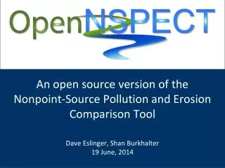
An open source version of the Nonpoint-Source Pollution and Erosion Comparison Tool. Dave Eslinger, Shan Burkhalter , Matt Pendleton 10 May, 2012. Outline. Background Getting started Installation Activation Basic analysis Advanced analysis. Background. Why this tool? Why open source?

E N D
An open source version of the Nonpoint-Source Pollution and Erosion Comparison Tool Dave Eslinger, Shan Burkhalter, Matt Pendleton 10 May, 2012
Outline • Background • Getting started • Installation • Activation • Basic analysis • Advanced analysis
Background • Why this tool? • Why open source? • What does OpenNSPECT do? • What do you need to run it? • What does it produce? • Who else has used it? • How can you get involved?
Why this tool? • Hawai‘i managers needed a simple, quick screening tool • Usable in a public setting • Could run on a laptop • Initially applied in Wai‘anae region in O‘ahu, Hawai‘i • Pressure from residential development • Sensitive coastal habitats • 2004: Esri ArcGIS 8.x extension • Updated for 9.0, 9.1, 9.2, 9.3 • 2011: OpenNSPECT
Why Open Source? • N-SPECT Requirements • Esri ArcGIS Desktop • Spatial Analyst Extension • ArcGIS 10 changes • Customer requests • “easy, online and free” • MapWindow • GeoTools 2007 • EPA BASINS
Open Source and ESRI versions • Strengths • Speed • “Free” • Community support • Weaknesses • Different program • learning curve, anxiety, distrust • Some features missing • Community support
What does OpenNSPECT do? • Water quality screening tool • Spatially distributed (raster-based) pollutant and sediment yield model • Compares the effects of different land cover and land use scenarios on total yields • User friendly graphical interface within a GIS environment
Processes Simulated • Topography determines flow direction and slope • Soil characteristics, land cover, andprecipitation determine runoff • Runoff, land cover, and pollutant coefficients determine pollutant loads • Runoff, topography, soil characteristics, and land coverdetermine sediment loads
Uses Existing Approaches • Rainfall runoff • Soil Conservation Service (SCS) curve number technique • Nonpoint pollutant • Event mean concentration technique • Sediment erosion • Universal Soil Loss Equation (USLE) • Modified (MUSLE) • Revised (RUSLE)
Assumptions/Limitations • Omitted processes • Stormwater drainage • Stream diversions • Snowmelt • Landslides • No time component for • Runoff dynamics • Sediment redeposition • Pollutant dynamics Source: NASA Earth Science Enterprise
What do you need to run it? • National sources* • Land cover data • Topography • Precipitation • Soils data • Pollutant coefficients • Rainfall erosivity • Local sources • Water quality standards • Additional pollutant coefficients *Local “tuning” improves accuracy
Topography • Defines flow direction, stream networks, watersheds • Default • U.S. Geological Survey (USGS) 30 m resolution digital elevation model • Resolution impacts processing speed and file size
Land Cover • Foundation for runoff quantity, sediment yield, pollutant yield • Default • Coastal Change Analysis Program (C-CAP) • 30 m resolution • Flexible • Can easily substitute any land cover grid
Soils • Runoff and erosion estimates are dependent upon soils and land cover • Default • SSURGO soils† • County level resolution • Infiltration rate • Hydrologic group • Soil erodibility • K-factor † Soil Survey Geographic Database provided by the Natural Resources Conservation Service
Precipitation • Derived from point estimates or modeled • OSU PRISM data • Annual average • Single event rainfall
Pollutants • Pollutant coefficients • Event mean concentrations • Land cover specific • Defaults • Nitrogen • Phosphorus • Lead • Zinc • User–definable • New pollutants • New coefficients • Different criteria
What does it produce? • Runoff volume • Accumulated runoff • Sediment yield • Accumulated sediment load • Pollutant yield • Accumulated pollutant load • Pollutant concentration
Flow directions derived from topography Precipitation grid provides amount of rainfall Uses soils and land cover data to estimate volume of runoff Validated Baseline Runoff Flow direction
Estimates total annual sediment load delivered to coast Provides a conservative estimate A “worst-case” scenario Baseline Erosion
Baseline Nitrogen • Estimates total annual pollutant load delivered to coast • Focuses attention on source areas
Baseline Nitrogen • Estimates total annual pollutant concentration • Focuses attention on source areas
Who else is using it? • Pelekane Bay, Hawaii • Sediments from extreme events.
Who else is using it? • Kingston Lake Watershed Association, near Conway, SC • Nutrient loads under different growth scenarios
Getting involved • OpenNSPECT: • Nspect.codeplex.com • MapWindow.org • Esri N-SPECT: • www.csc.noaa.gov/nspect • NSPECT listserver • https://csc.noaa.gov/mailman/listinfo/n-spect-community
Project Contacts: Dave Eslinger, Project lead Dave.Eslinger@noaa.gov 843-740-1270 Shan Burkhalter Shan.Burkhalter@noaa.gov 843-740-1275 Matt Pendleton Matt.Pendleton@noaa.gov 843-740-1196 Questions?
Example Application • Makaha Valley, O‘ahu, Hawai‘i • Annual time scale • “What-if” scenario • Baseline • Land cover change • New residential development • Comparison
Land Cover Change Scenario • Develop a subdivision • Change scrub/shrub vegetation to low intensity development
Nitrogen (Pre-Change) • Baseline • Low nitrogen runoff • Add scenario
Nitrogen (Post-Change) • Compare baseline estimate to the new estimated load • Can calculate the difference in annual nitrogen load
Download OpenNSPECT: www.csc.noaa.gov/nspect Today’s Trainer: Dave Eslinger Dave.Eslinger@noaa.gov 843-740-1270 Project Contacts: Dave Eslinger, Project lead Dave.Eslinger@noaa.gov 843-740-1270 Shan Burkhalter Shan.Burkhalter@noaa.gov 843-740-1275 Matt Pendleton Matt.Pendleton@noaa.gov 843-740-1196 Questions?
Outline • Background • Getting started • Installation • Activation • Import new data • Basic analysis • Advanced analysis
MapWindow GIS • Free • Open-source • Desktop GIS • Developer driven applications (plugins) • OpenNSPECT • BASINS • 3D Viewer
Installation • Two-part installation • MapWindowGIS • OpenNSPECT • Contents of C:\NSPECT • TODAY adding • HI_Sample_Data • Unzip into C:\NSPECT\
Activation • Open MapWindowGIS • MapWindow Pull-Down Menu, select Plug-ins > OpenNSPECT
Import Landcover • OpenNSPECT/ Advanced Settings/Land Cover Types • Options/Import • Browse to coefficient file • Import with new LC name
Import Pollutants • OpenNSPECT/ Advanced Pollutants • Pick Pollutant • Coefficients /Import • Pick LC type • Browse to coefficient file • Import with new Coefficient Set name
Text change in Tutorial • Change both “NitSet” to “NitSet05” • Page 4 • Page 13
Outline • Background • Getting started • Basic analysis • Baseline • Exercise 1 - Accumulated effects • Exercise 2 - Local effects • Conclusion • Advanced analysis
Basic Analysis • Baseline analyses • Objective • Run a basic analysis with OpenNSPECT and produce baseline runoff, erosion, and pollutant load data sets for an annual time scale. • Important Learning Objectives: • Gain familiarity with the OpenNSPECT user interface. • Learn which data sets are necessary to run the model. • Understand the properties associated with the Pollutants tab. • Understand the properties associated with the Erosion tab. • Understand the function of the Local Effects Only option. • Learn to visually assess the data output.
Exercise 1 • Baseline analysis (accumulated effects) • Accumulated runoff, nonpoint source pollutants, and eroded sediments are estimated. • Accumulated effects include: • Expected pollutant or sediment concentration at a cell. • Contributions from upstream cells. • Page 3
Exercise 2 • Baseline analysis (local effects) • Local effects of runoff, nonpoint source pollution, and erosion are estimated. • Local effects include expected pollutant or sediment concentration at a cell without upslope contributions. • Page 5
Exercises 1 and 2 Results • Baseline runoff, sediment loads, and nitrogen concentrations (accumulated and nonaccumulated) • Model outputs are representative of the landscape conditions during the time at which the input data was collected. • Visual interpretation • Topography was associated with the shape and density of drainage networks. • Land cover types were associated with various degrees of sediment and pollutant loads.
Outline • Background • Getting started • Basic analysis • Advanced analysis • Management scenario • Exercise 3 – Accumulated and Local effects • Alternative land use • Exercise 4 - Accumulated effects
Advanced Analysis • Management scenario analyses • Objective • Run an analysis that incorporates a hypothetical management scenario and examines the potential changes to runoff, erosion, and pollution. • Important Learning Objectives: • Understand the properties associated with the Management Scenarios tab. • Learn to incorporate a management scenario. • Learn to quantitatively evaluate the data output. • Understand the relative contributions of different land cover classes to nonpoint source pollution.
Exercises 3 • Management scenario • Integration of a hypothetical land management scenario • Grassland and scrub/shrub converted to low intensity developed land. • Local effects of runoff, nonpoint-source pollution, and erosion are estimated. • Accumulated effects of runoff, nonpoint-source pollution, and erosion are estimated. • Comparison to baseline results. • Page 7
Exercise 3 Results Baseline • Nitrogen yields (mg) • Baseline conditions • Low density residential management scenario • Difference between A and B • The 0.2 km2 development is predicted to yield an additional 86.7 kilograms of nitrogen under the alternative land management scenario (a 138 percent increase). Management Comparison % Change
Exercise 3 Results • Nitrogen yields (mg) • This translates to a 0.5 percent increase in the accumulated nitrogen load for the entire 14.1 km2 watershed.
Advanced Analysis • Alternative land use scenario analysis • Objective • Run an analysis with a new land use scenario and produce modified runoff, erosion, and pollutant load data sets for an annual timescale. • Important learning objectives: • Understand the properties associated with the Land Use tab. • Learn to parameterize a new land use scenario. • Learn to quantitatively evaluate the data output.