Download
1 / 14
210 likes | 441 Views
Boltzmann Machine (BM) (§6.4). Hopfield model + hidden nodes + simulated annealing BM Architecture a set of visible nodes: nodes can be accessed from outside a set of hidden nodes: adding hidden nodes to increase the computing power

E N D
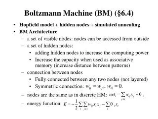
Boltzmann Machine (BM) (§6.4) • Hopfield model + hidden nodes + simulated annealing • BM Architecture • a set of visible nodes: nodes can be accessed from outside • a set of hidden nodes: • adding hidden nodes to increase the computing power • Increase the capacity when used as associative memory (increase distance between patterns) • connection between nodes • Fully connected between any two nodes (not layered) • Symmetric connection: • nodes are the same as in discrete HM: • energy function:
BM computing (SA), with a given set of weights 1. Apply an input pattern to the visible nodes. • some components may be missing or corrupted ---pattern completion/correction; • some components may be permanently clamped to the input values (as recall key or problem input parameters). 2. Assign randomly 0/1 to all unknown nodes ( including all hidden nodes and visible nodes with missing input values). 3. Perform SA process according to a given cooling schedule. Specifically, at any given temperature T. a random picked non-clamped node i is assigned value of 1 with probability , and 0 with probability
hidden 2 3 visible 1 • BM learning ( obtaining weights from exemplars) • what is to be learned? • probability distribution of visible vectors in the environment. • exemplars: assuming randomly drawn from the entire population of possible visible vectors. • construct a model of the environment that has the same prob. distri. of visible nodes as the one in the exemplar set. • There may be many models satisfying this condition • because the model involves hidden nodes. Infinite ways to assign prob. to individual states • let the model have equal probability of theses states (max. entropy); • let these states obey B-G distribution (prob. proportional to energy).
BM Learning rule: : the set of exemplars ( visible vectors) : the set of vectors appearing on the hidden nodes two phases: • clamping phase: each exemplar is clamped to visible nodes. (associate a state Hb to Va) • free-run phase: none of the visible node is clamped (make (Hb , Va) pair a min. energy state) : probability that exemplar is applied in clamping phase (determined by the training set) : probability that the system is stabilized with at visible nodes in free-run (determined by the model)
learning is to construct the weight matrix such that is as close to as possible. • A measure of the closeness of two probability distributions (called maximum likelihood, asymmetric divergence, or cross-entropy): • It can be shown • BM learning takes the gradient descent approach to minimal G
BM Learning algorithm 1. compute 1.1. clamp one training vector to the visible nodes of the network 1.2. anneal the network according to the annealing schedule until equilibrium is reached at a pre-set low temperature T1 (close to 0). 1.3. continue to run the network for many cycles at T1. After each cycle, determine which pairs of connected node are “on” simultaneously. 1.4. average the co-occurrence results from 1.3 1.5. repeat steps 1.1 to 1.4 for all training vectors and average the co-occurrence results to estimate for each pair of connected nodes.
2. Compute the same steps as 1.1 to 1.5 except no visible node is clamped. 3. Calculate and apply weight change 4. Repeat steps 1 to 3 until is sufficiently small.
Comments on BM learning • BM is a stochastic machine not a deterministic one. • It has higher representative/computation power than HM+SA (due to the existence of hidden nodes). • Since learning takes gradient descent approach, only local optimal result is guaranteed (G may not be reduced to 0). • Learning can be extremely slow, due to repeated SA involved • Speed up: • Hardware implementation • Mean field theory: turning BM to deterministic by replacing random variables xi by its expected values
Evolutionary Computing (§7.5) • Another expensive method for global optimization • Stochastic state-space search emulating biological evolutionary mechanisms • Biological reproduction • Most properties of offspring are inherited from parents, some are resulted from random perturbation of gene structures (mutation) • Each parent contributes different part of the offspring’s chromosome structure (cross-over) • Biological evolution: survival of the fittest • Individuals of greater fitness have more offspring • Genes that contribute to greater fitness are more predominant in the population
population selection of parents for reproduction (based on a fitness function) parents reproduction (cross-over + mutation) next generation of population Overview • Variations of evolutionary computing: • Genetic algorithm (relying more on cross-over) • Genetic programming • Evolutionary programming (mutation is the primary operation) • Evolutionary strategies (using real-value vectors and self-adapting variables (e.g., covariance))
Basics • Individual: • corresponding to a state • represented as a string of symbols (genes and chromosomes), similar to a feature vector. • Population of individuals (at current generation) • Fitness function f: estimates the goodness of individuals • Selection for reproduction: • randomly select a pair of parents from the current population • individuals with higher fitness function values have higher probabilities to be selected • Reproduction: • crossover allows offspring to inherit and combine good features from their parents • mutation (randomly altering genes) may produce new (hopefully good) features • Bad individuals are throw away when the limit of population size is reached
Comments • Initialization: • Random, • Plus sub-optimal states generated from fast heuristic methods • Termination: • All individual in the population are almost identical (converged) • Fitness values stop to improve over many generations • Pre-set max # of iterations exceeded • To ensure good results • Population size must be large (but how large?) • Allow it to run for a long time (but how long?)