Download

1 / 53
600 likes | 1.05k Views
Image Segmentation. Rob Atlas Nick Bridle Evan Radkoff. Image Segmentation. Separate an image into sets of pixels which represent some structure in the image Main application is object and boundary detection. High Level Overview of Papers. Image Segmentation. Local approaches. Graph cuts.

E N D
Image Segmentation Rob Atlas Nick Bridle Evan Radkoff
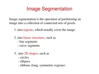
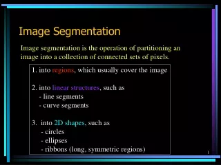
Image Segmentation Separate an image into sets of pixels which represent some structure in the image Main application is object and boundary detection
High Level Overview of Papers Image Segmentation Local approaches Graph cuts Mean Shift Normalized Cuts Shi and Malik, 2000 Comaniciu et al., 1999 Interactive Cuts Rother et al., 2004 Li et al., 2004
Mean Shift Analysis Dorin Comaniciu, Peter Meer Rutgers University, ICCV 1999
Spatial-Range Domain Spatial domain: pixel locations Range domain: intensity values Spatial-Range domain: concatenation of the two { x, y, R, G, B } Parameters: ∂s: Spatial domain normalization ∂r: Range domain normalization { x / ∂s , y / ∂s , R / ∂r , G / ∂r , B / ∂r } 5 dimensions for RGB, 3 for grayscale
Kernel Density Estimate For n points {xi}i=1..n in a d-dimensional Euclidean space with kernel function K(x) and window radius h:
Epanechnikov Kernel cd : volume of the unit d-dimensional sphere
Estimating the Density Gradient Goal: where Sh is a hypersphere containing nx data points
Mean Shift Vector Vector with a direction towards the largest increase in density, thus leading to a local density maximum.
Mean Shift Procedure 1) Compute the mean shift vector Mh(x) 2) Translate the window Sh(x) by Mh(x) 3) If not converged, go to step 1. Mathematically guaranteed to converge
Applying Mean Shift to Images Spatial-Range Domain: { x / ∂s , y / ∂s , R / ∂r , G / ∂r , B / ∂r } The authors apply the mean shift procedure to all points in the spatial-range domain. Two applications: Filtering, Segmentation Two parameters: spatial resolution and range resolution
Mean Shift Filtering xi: source pixel zi: filtered pixel for each xi apply the mean shift procedure on xi to find the convergence point yi spacial domain of zi = spacial domain of xi range domain of zi = range domain of yi
Segmentation Instead of changing pixels ranges (colors), group them by which point their mean shift procedure converges to.
Advantages: No oversight required Preserves detail when appropriate Disadvantages: Cannot choose how many segments are made
Normalized Cuts and Image Segmentation Shi and Malik, 2000 ...
Basic Idea Treat image segmentation as a graph-partitioning problem Big Questions: 1. How do we define a good partitioning? 2. How do we do partition efficiently?
Images as a graph G=(V,E) Vertices: pixels Edges: similarity
Graph cuts Assumes: Graph is fully connected Given: G=(V,E) Do: Create disjoint vertex sets A, B s.t. and
Similarity metric Weight between edges in graph: X(i): Location of pixel i F(i): Feature vector describing pixel i Simple case - F(i)=1 for segmenting points Intensity, color, texture , : Parameters
2-way graph cut Minimize: Existing efficient methods for optimal 2-way cut
Recursive minimum cuts Iteratively bipartition graph according to minimum cut (Wu and Leahy, 1993) The problem: favors small clusters
Intuition for normalized cuts Want to minimize cut score But, we also want to partition out larger areas with more connections So, what we're really interested in is the proportion of total weights that we are cutting for each segment
Normalized cuts Goal: partition into disassociated groups
Minimizing association between groups ~ maximizing association within groups
Computational complexity Minimizing normalized cut: NP-complete Can compute approximate solution by solving a generalized eigenvalue problem
Eigenvalue system D - diagonal matrix of the total weight from each node to every other W - matrix of weights between nodes y - eigenvectors lambda - eigenvalues However, this is not in standard form for solving
A solvable representation First eigenvector (eigenvalue=0):
Second smallest eigenvalue describes solution Remember, the smallest eigenvalue is 0
Recursive two-way Ncut Third, fourth, etc eigenvalues correspond to eigenvectors that subdivide the existing graphs However, error accumulates with each Better to recompute partitioning on each subgraph iteratively
Segmentation Algorithm 1. Create weighted graph G=(V,E) 2. Solve and take the eigenvector with the second smallest eigenvalue 3. Bipartition the graph with this eigenvector 4. If Ncut is below threshold value, recursively partition each segment
Partitioning by an eigenvector The partitioning eigenvector contains one continuous value per pixel Since these are continuous, not discrete, they don't directly tell us which points are in which segment Instead, we try different cutoffs, and select the one that produces the minimal NCut value
Interactive Graph Cuts User can provide hints about where the objects are in the scene Ideally, the less work the user has to do, the better
Foreground Extraction Goal is to partition the pixels into two sets: foreground and background
Foreground Extraction Given pixel intensity values Output set of alphas which determine how much each pixel belongs to the foreground "Hard segmentation": "Soft segmentation":
GrabCut Rother et al., SIGGRAPH 2004
GrabCut: Handling Color Images Previous work: histogram of gray values for foreground and background GrabCut: - histograms are intractable for color - instead use Gaussian Mixture Model (GMM) to represent the distribution of color
GrabCut: Border Matting Perform hard segmentation on image, and then relax alpha values on the border of the object
Lazy Snapping Li et al., SIGGRAPH 2004
Lazy Snapping: Energy Function Minimize the Gibbs energy function Run k-means clustering on foreground and background points E1 defined in terms of these mean colors:
Lazy Snapping: Speeding it up Speed is crucial for a responsive user experience Use the watershed algorithm to divide the image into small approximately constant patches, then do graph cut using these as the nodes