Unlocking the Power of SAS: Data Management and Analysis Techniques
This guide explores the diverse capabilities of SAS software for data management and analysis, covering key techniques such as linear programming, econometrics, data mining, and statistical analysis. Learn how to effectively handle various data types, including panel data and relational databases, and understand the difference between DATA and PROC steps in SAS. Discover practical examples and routines for manipulating, transforming, and reporting data, essential for maximizing your analytical workflows and improving decision-making processes in any organization.

Unlocking the Power of SAS: Data Management and Analysis Techniques
E N D
Presentation Transcript
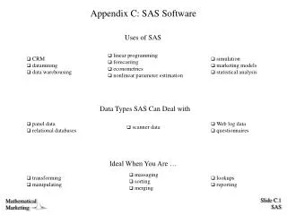
Appendix C: SAS Software Uses of SAS • linear programming • forecasting • econometrics • nonlinear parameter estimation • CRM • datamining • data warehousing • simulation • marketing models • statistical analysis Data Types SAS Can Deal with • panel data • relational databases • Web log data • questionnaires • scanner data Ideal When You Are … • massaging • sorting • merging • transforming • manipulating • lookups • reporting
Two Types of SAS Routines • DATA Steps • Read and Write Data • Create a SAS dataset • Manipulate and Transform Data • Open-Ended - Procedural Language • Presence of INPUT statement creates a Loop • PROC Steps • Analyze Data • Canned or Preprogrammed Input and Output
A Simple Example data my_study ; input id gender $ green recycle ; cards ; 001 m 4 2 002 m 3 1 003 f 3 2 ••• ••• ••• ••• ; proc reg data=my_study ; class gender ; model recycle = green gender ;
The Sequence Depends on the Need data step to read in scanner data; data step to read in panel data ; data step to merge scanner and panel records ; data step to change the level of analysis to the household ; proc step to create covariance matrix ; data step to write covariance matrix in LISREL compatable format ;
The INPUT Statement - Character Data • List input $ after a variable - character var input last_name $ first_name $ initial $ ; • Formatted input $w. after a variable input last_name $22. first_name $22. initial $1. • Column input $ start-column - end-column input last_name $ 1 - 22 first_name $ 23 - 45 initial $ 46 ;
The INPUT Statement - Numeric Data • List input input score_1 score_2 score_3 ; • Formatted input w.d (field width and number of digits after an implied decimal point) after a variable input score_1 $10. score_2 $10. score_3 10. • Column input $ start-column - end-column input score_1 1 - 10 score_2 11 - 20 score_3 21 - 30 ;
Grouped INPUT Statements input (var1-var3) (10. 10. 10.) ; input (var1-var3) (3*10.) ; input (var1-var3) (10.) ; input (name var1-var3) ($10. 3*5.1) ;
The Column Pointer in the INPUT Statement input @3 var1 10. ; input more @ ; if more then input @15 x1 x2 ; input @12 x1 5. +3 x2 ;
Documenting INPUT Statements input @4 green1 4. /* greeness scale first item */ @9 green2 4. /* greeness scale 2nd item */ @20 aware1 5. /* awareness scale first item */ @20 aware2 5. ; /* awareness scale 2nd item */
The Line Pointer input x1 x2 x3 / x4 x4 x6 ; input x1 x2 x3 #2 x4 x5 x6 ; input x1 x2 x3 #2 x4 x5 x6 ;
Reading an External File on Unix data ; filename raw_sem 'my_garnet_disk_file.data' ; infile raw_sem ; input a b etc. ;
The PUT Statement put x1 x2 x3 @ ; input x4 ; put x4 ; put x1 #2 x2 ; put x1 / x2 ; put _all_ ; put a= b= ; put _infile_ ; put _page_ ; col1 = 22 ; col2 = 14 ; put @col1 var245 @col2 var246 ;
Copying Raw Data data _null_ ; infile in ; outfile out ; input ; put _infile_ ;
SAS Constants '21Dec1981'D 'Charles F. Hofacker' 492992.1223
Assignment Statement x = a + b ; y = x / 2. ; prob = 1 - exp(-z**2/2) ;
The SAS Array Statement array y {20} y1-y20 ; do i = 1 to 20 ; y{i} = 11 - y{i} ; end ;
The Sum Statement variable+expression ; retain variable ; variable = variable + expression ; n+1 ; cumulated + x ;
IF Statement if a >= 45 then a = 45 ; if 0 < age < 1 then age = 1 ; if a = 2 or b = 3 then c = 1 ; if a = 2 and b = 3 then c = 1 ; if major = "FIN" ; if major = "FIN" then do ; a = 1 ; b = 2 ; end ;
More IF Statement Expressions name ne 'smith' name ~= 'smith' x eq 1 or x eq 2 x=1 | x=2 a <= b | a >= c a le b or a le c a1 and a2 or a3 (a1 and a2) or a3 then etc ; if
Concatenating Datasets Sequentially first: id x y 1 2 3 2 1 2 3 3 1 second: id x y 4 3 2 5 2 1 6 1 1 data both ; set first second ; both: id x y 1 2 3 2 1 2 3 3 1 4 3 2 5 2 1 6 1 1
Interleaving Two Datasets proc sort data=store1 ; by date ; proc sort data=store2 ; by date ; data both ; set store1 store2 ; by date ;
Concatenating Datasets Horizontally left: id y1 y2 1 2 3 2 1 2 3 3 1 right: id x1 x2 1 3 2 2 2 1 3 1 1 data both ; merge left right ; both: id y1 y2 x1 x2 1 2 3 3 2 2 1 2 2 1 3 3 1 1 1
Table LookUp table: part desc 0011 hammer 0012 nail 0013 bow database: id part 1 0011 2 0011 3 0013 proc sort data=database out=sorted by part ; data both ; merge table sorted ; by part ; both: id part desc 1 0011 hammer 2 0011 hammer 3 0013 bow
Changing the Level of Analysis 1 Day Score Student 1 12 A 1 11 B 1 13 C 2 14 A 2 10 B 2 9 C Day Highest Student 1 13 C 2 14 A Before After
Changing the Level of Analysis 1FIRST. and LAST. Variable Modifiers proc sort data=log ; by day ; data find_highest ; retain hightest ; drop score ; set log ; by day ; if first.day then highest=. ; if score > highest then highest = score ; if lastday then output ;
Changing the Level of Analysis 2 Subject Time Score A 1 A1 A 2 A2 A 3 A3 B 1 B1 B 2 B2 B 3 B3 Subject Score1 Score2 Score3 A A1 A2 A3 B B1 B2 B3 Before After
Changing the Level of Analysis 2 data after ; keep subject score1 score2 score3 ; retain score1 score2 ; set before ; if time=1 then score1 = score ; else if time=2 then score2 = score ; else if time=3 then do ; score3 = score ; output ; end ;
The KEEP and DROP Statements keep a b f h ; drop x1-x99 ; data a(keep = a1 a2) b(keep = b1 b2) ; set x ; if blah then output a ; else output b ;
Changing the Level of Analysis 3Spreading Out an Observation Subject Score1 Score2 Score3 A A1 A2 A3 B B1 B2 B3 Subject Time Score A 1 A1 A 2 A2 A 3 A3 B 1 B1 B 2 B2 B 3 B3 Before After
Code for Change 3 data spread ; drop score1 score2 score3 ; set tight ; time = 1 ; score = score1 ; output ; time = 2 ; score = score2 ; output ; time = 3 ; score = score3 ; output ;
Use of the IN= Dataset Indicator data new ; set old1 (in=from_old1) old2 (in=from_old2) ; if from_old1 then … ; if from_old2 then … ;
Proc Summary for Aggregation • proc summary data=raw_purchases ; • by household ; • class brand ; • output out=household count=x x=y ; • VAR variable(s)</ WEIGHT=weight-variable>;
Using SAS for Simulations data monte_carlo ; keep y1 - y4 ; array y{4} y1 - y4 ; array loading{4} l1 - l4 ; array unique{4} u1 - u4 ; l1 = 1 ; l2 = .5 ; l3 = .5 ; l4 = .5 ; u1 = .2 ; u2 = .2 ; u3 = .2 ; u4 = .2 ; do subject = 1 to 100 ; eta = rannor(1921) ; do j = 1 to 4 ; y{j} = eta*loading{j} + unique{j}*rannor(2917) ; end ; output ; end ; proc calis data=monte_carlo ; etc. ; Simulation Loop