Download
1 / 27
270 likes | 388 Views
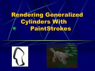
This article explores the rendering of generalized cylinders using paint strokes, a technique that extrudes a circular shape along a defined path, allowing variations in radius. It details the parametric functions that define visual attributes such as position, radius, color, opacity, and reflectance, which vary along the stroke. The use of Catmull-Rom splines to construct the paint stroke path and color interpolation across control points are discussed. The process also includes tessellation of the stroke into polygons, enabling realistic 3D rendering in graphical applications.

E N D
A generalized cylinder is the surface produced by extruding a circle along a path through space, allowing the circle's radius to vary along the path. • The essential properties of a paintstroke can be described with a one dimensional parametric function, ps(t). The components of this function are visual attributes that vary along the length of the paintstroke : position radius, colour, opacity, and reflectance.
pos(t) rad(t) ps(t) = colour(t) op(t) reflectance(t) The ps(t) function is defined by using a series of n2 control points, {cp0 , cp1 , …,cpn-1 }.
we define psm (t) as the section of ps(T) where T [a, b] such that ps(a) =cpm and ps(b) =cpm+1 . The new parameter, t [0,1], ranges over a single section of a paintstroke between a pair of neighbouring control points: psm (0) = cpm psm (1) = cpm+1 segment refers to a subset of a section.
The Pos Function posx(t) pos(t) = posy(t) posz(t) The function pos(t) defines the path that the paintstroke segment follows through R3 using the Catmull-Rom spline. Given the eye-space position values pm-1,pm, pm+1, and pm+2 of the control points, the Catmull-Rom spline extends from pm to pm+1, according to the equation :
As the figure shows, a Catmull-Rom spline is equivalent to a Hermite curve, such that the tangent vector at each inner control point joins the two surrounding control points. Another term we shall refer to is the view vector, dened as the unit vector from the viewer (at the origin) to a point on the paintstroke. Thus, view(t) = pos(t)/||pos(t)||.
The Radius - The function rad(t) defines the thickness of the segment, measured orthogonally to the tangent vector of the path, pos’(t). The radius function is defined as a Catmull-Rom spline, precisely like each component of pos(t). The model supplies a set of radiuses { r0,r1,…, rn-1} at each control point .
The Color - colorr(t) color(t) = colorg(t) colorb(t) A color value is assigned at each control point, and the color(t) function interpolates linearly between these values, along the spine of the paintstroke. Given the set of (r, g, b) color points {c0,c1,…,cn-1} , the equation for the interpolated color value between control points cm and cm+1 is : colorm(t) = (1-t)cm + tcm+1 Black Control point White Control Point
Tessellating the Paintstroke-or polygonizing it Traditional tessellation schemes subdivide a surface into a set of world-space Polygons . Although , The paintstroke directly polygonizes the screen projection of a generalized cylinder. This is what makes the name “paintstroke" appropriate to this primitive: a painter drawing a three-dimensional tube with a single stroke of the paintbrush . Each section of the paintstroke, bounded by control points {cp0, cp1} , {cp1, cp2} … {cpn-2, cpn-1} , is rendered individually. The following two phases will subdivide the section, first along its length, and then along its breadth. The lengthwise subdivision breaks the section into segments, each of which is then divided along its breadth to ultimately produce a set of polygons. That completes the tessellation.
Lengthwise Subdivision the section between each pair of adjacent control points is recursively subdivided in half into pairs of segments until the subdivision criterion for all the segments has been satisfied. Whenever a segment is subdivided, the split occurs at the parametric midpoint, i.e. at ps(0.5). The two halves are then recursively subdivided in the same manner until no further subdivisions are required. A paintstroke segment ps(t) for t[a,b] a < b is either subdivided or advances to the next phase, depending on the behavior of its pos(t) and rad(t) components.
Position Constraint I The first position constraint is based on the angle between the two dimensional tangent vectors pos’scr (a) and pos’scr (b). These are the (x,y) screen-space projections of the derivative pos’(t) at the segment's endpoints, t = a and t = b. If > max , the constraint forces a subdivision. max (0°,90°) as described in the next page. The values pos’scr (a) and pos’scr (b) are obtained by analytically dierentiating the function posscr(t), the screen-projection of the paintstroke's path.
The next step is to normalize pos’scr (a) and pos’scr (b), and then compute their dot product, which yields cos. If this value is negative, then exceeds the maximum value of max (90°) so we subdivide the segment . Otherwise, we need to determine max . We begin by finding the segment's maximum length d, defined as the distance between the two outside points oa and ob, which are the points lying on the outside boundary of the segment at t = a and t = b. The outside point oa is computed by displacing the position point posscr(a) by one of the two vectors perpendicular to pos’scr (a) , namely : pos’scr y(a) or -pos’scr y(a) -pos’scr x(a) pos’scr x(a) That has been normalized and scaled by the length of the screen-projected radius.To determine which of the two vectors points toward the outside of the paintstroke's curvature, we apply a test based on pos’’scr(a), because the second derivative vector always points toward the center of curvature.
The same algorithm is applied to obtain ob. Then d which is the distance between oa and ob is found . max is obtained by the equation - cos² max = d² d² + tol² tol is a user-defined parameter which causes more or less segmentization. Now , if > max we divide the segment , else , we proceed to the next phase.
Position Constraint Il The second position constraint maintains a desired degree of linearity in the z Component of pos(t). This is necessary to ensure that a curved segment is adequately subdivided even when viewed from an angle that makes its screen projection close to linear. In such a situation, Position Constraint I would allow the entire segment to be rendered without any subdivision, regardless of its true curvature. Although the rendered image would have the correct shape, it would fail to express the true variation in the surface normals along the segment. To implement this constraint, we begin by computing over the interval [a,b] the exact average values of posz(t) and its linear interpolant. The absolute difference between the two is a measure of posz(t)'s nonlinearity. If the result is Smaller than tolz (user-defined parameter) than a segmentization occurs else we proceed onto the next phase.
The Radius Constraint The radius constraint ensures a smooth lengthwise variation in the radius of a segment. It is precisely analogous to Position Constraint II, relying on the average difference between the rad(t) function and its linear interpolant. The simplified equation for this constraint is :
Breadthwise Subdivision After a segment has been sufficiently shortened by lengthwise subdivision, it is finally tessellated into polygons along its breadth.This involves dividing it into a ring of polygons which tile the truncated cone that the segment represents. The specifics of a paintstroke's breadthwise tessellation depend on its quality level.Each paintstroke bears one of three possible quality levels, numbered 0, 1, and 2. a quality-zero segment is tessellated into a single polygon that always faces the viewer, a quality-one segment into two on each side (the viewer's side and the one opposite to it), and a quality-two segment into four on each side.
2 polygons 1 polygon 4 polygons
Quality Level 0 - the entire segment becomes a single quadrilateral with vertices along the edges of the paintstroke, corresponding to the silhouette of the generalized cylinder. -The shading and lightening is inaccurate. -Can’t be viewd head-on. Quality Level 1 - the viewer's side of the segment is divided into two equal- sized quadrilaterals that have a common edge along the middle of the segment. improves the appearance of a lighted segment,can be viewed head-on, - reveal their quadrilateral cross-section if their path is sufficiently straight. Quality Level 2 - produce the highest quality images, both in their shading and in their appearance when viewed head-on. - generate four polygons per segment.
Determining the Polygon Vertices To obtain a paintstroke polygon's vertices, There’s a need to determine the vectors which all originate at pos(t), radiating outward. These are the out vectors: outedge(t) - points to one of the segment's two lengthwise silhouette edges. outcenter(t) - reaches the breadthwise center of the segment.
Vertices along the edges are now computed as : pos(t)+outedge(t) pos(t)- outedge(t) For quality-zero paintstrokes, these are the only vertices used. For higher quality levels, the center vertex on the side of the segment facing the viewer is given by pos(t) +outcenter(t). For quality2 paintstrokes, the remaining four vertices are computed in the same manner, outmid1(t) and outmid2(t) as described previously. The vertices are computed at both endpoints (a,b) of the segment, yielding a ringof quadrilaterals.
Computing the Normals Each normal vector is equal to its corresponding out(t) vector plus an adjustment vector adj(t) in the direction of pos’(t), whose norm is determined by the derivatives of the radius and position : adj(t) = - rad’(t)pos’(t) ||pos’(t)||² out(t) vectors define the breadthwise normal varia- tion of a paintstroke , while the adj(t) vector Represents the lengthwise normal variation, determined by the behavior of the paintstroke's radius.Then the Normal vector at each vertex is - Normal = out”correspond”(t) + adj(t) The normals within the interior of a polygon are derived by bilinearly interpolating the (x, y, z) com- ponents of the vertex normals across the polygon's screen-space projection.
Conclusions The purpose of this paper was to provide an efficient means of rendering generalized cylinders at precisely small and medium scales. By applying a view-adaptive tessellation algorithm that exploits the simplicity and symmetry of the generalized cylinder's screen-space projection, paintstrokes are able to accurately approximate furry surfaces using much fewer polygons than competing methods, producing savings in both rendering speed and memory consumption.
Bibliography • http://www.dgp.utoronto.ca/people/ivan/research/research.html#anims • http://www.dgp.utoronto.ca/people/ivan/research/sketch.pdf SIGGRAPH '97 Technical Sketch, Aug. 1997 • http://www.dgp.utoronto.ca/people/ivan/research/gi98.pdf Graphics Interface '98, June 1998 • http://www.dgp.utoronto.ca/people/ivan/research/thesis.pdf