Climate Models : Past to Present
420 likes | 722 Views
Climate Models : Past to Present. V.Vidyunmala Ph.D Student Student’s Seminar Series. Plan of Talk. Climate System Scales of Climate System Evolution of models Comparison of AMIP-CMIP results Model Sensitivities. Climate System:.

Climate Models : Past to Present
E N D
Presentation Transcript
Climate Models: Past to Present V.Vidyunmala Ph.D Student Student’s Seminar Series
Plan of Talk • Climate System • Scales of Climate System • Evolution of models • Comparison of AMIP-CMIP results • Model Sensitivities
Climate System: Climate system consists of atmosphere, hydrosphere, cryosphere, lithosphere and biosphere
Positive Feedback Greenhouse effect of water vapour and atmospheric temperature Albedo of snow and ice cover and atmospheric temperature Greenhouse effect of CO2 and the surface air temperature Negative Feedback Equator-to-pole temperature difference and the meridional heat transport Soil humidity and albedo of land surface Air temperature and cloudiness Feedbacks mechanisms in Climate: Climate processes are mainly forced by external and internal forcing mechanism External Forcing Solar forcing Internal Forcing Determined by the existence of feedbacks
Scales of temporal Variability of the Climate System: Climate system oscillation are found to have large temporal variability • Small scale oscillations : fraction of second to several minutes • Meso-scale oscillations : several minutes to several hours • Synoptic scale oscillations : several hours to several days in atmosphere and weeks in ocean • Global variations : weeks to months • Seasonal Variations : annual periods • Inter-annual Variations : periods of several years • Intra-centennial variations : periods of tens of years • Inter-centennial Variations : periods of several centuries • Long-Period Oscillations : periods of tens of thousands of years
Equilibration Time of the Climate System: Equilibration Time is the response time (or) relaxation time of the components of the climate system
What are models ? And why do we use them? “A climate model is a mathematical representation of the physical processes that determine climate” To gain quantitative insights into the behavior of the earth system. Models are natural extensions of theory: Theory : Analytic solutions Models : Numerical Solutions
Are these models Complex or Simple Box (1976) : “ ….all models are wrong some are useful. Accepting this principle, the job is not so much in search of the true model but to select a model that is appropriate for the problem in hand”. A useful model is not the one which is true but the one that is informative – Feldstein, 1982 Models are simplifications of the complexity of the nature Lastly, Models should be as simple as possible but not simpler - Einstein
Components of Climate Model: The main components of a climate model are: The way in which the input and absorption of solar radiation and the emission of infrared radiation are handled The movement of energy around the globe (from low latitude to high latitude) and vertical movements( convection) Inclusion of land/ocean/ice and the resultant change in albedo, emissivity, and surface-atmosphere exchanges. Radiation : Dynamics : Surface Processes :
Types of Climate models: Energy balance models (EBMs)are one-dimensional models predicting the variation of surface temperature with latitude. One-dimensional Radiative-Convective models (RCs)they compute the vertical temperature profile by explicit modelling of the radiative processes and a convective-adjustment which reestablishes a predetermined lapse rate Two-dimensional Statistical dynamical models (2D-SDs),they deal with surface processes and dynamics in a zonally averaged framework and have a vertically resolved atmosphere General Circulation Models (GCMs),these are three dimensional nature models of atmosphere/ocean with all the physics and dynamics included
Decade and landmark papers Climate model status < 1969 Richardson (1922) Manabe and Moller (1961) Manabe and Strickler (1965) Adem (1965) 1969-1981 Sellers (1969) Budyko (1969) Manabe and Bryan (1969) Green (1970) Stone (1973) Manabe and Wetherald (1975) CLIMAP (1981) Hansen et al (1981) 1981-1999 Sellers et al (1986) Oort and Peixoto (1983) Luther et al (1988) Houghton et al (1990) Semtner and Chervin (1992) Flato and Hibler (1992) Cubasch (1994) 1999- above First weather forecast by numerical calculation Extended numerical weather forecasts RC models developed Low resolution thermodynamics model developed Dynamics and radiation virtually separate EBMs newly described Multi-layer ocean added to GCMs SD models developed Greenhouse modeling with GCMs Paleo datasets first employed for validation GCMs becoming the predominant model type Surge in computation power and model type Satellite generated global observation Model Intercomparison suggested Simpler models required by IPCC OAGCMs established but need for flux correction Sea-ice and land surface component evolving First ocean-atmosphere coupled ensemble Past Climate simulation re-emerging for testing Model Intercomparison project for Atmosphere, Land and Ocean and Coupled models. etc. Historical Evolution of Climate Models
Energy Balance Models: Simple Energy Balance Model If we consider each latitude zone independently Disadvantages of 1-D EBM: They are sensitive to changes in solar constant and albedo.
There are two other types of EBMs : • A simple box model of the ocean-atmosphere : In this it is a system of four components, two atmosphere over ocean and land and a oceanic mixed layer and deeper different ocean. The heating of the mixed layer is calculated by assuming a constant depth in which the temperature difference changes due to thermal forcing, atmospheric feedback and leakage of energy permitted into underlying water. 2. A coupled atmosphere,land and ocean energy balance box model:It includes the polar sinking of oceanic water into deep oceans. Disadvantages: Hemispherically averagedcloud fraction is prescribed as seasonal varying feature. We cannot incorporate temperature of surface albedo feedback since land is hemispherically averaged
Radiative-Convective Models They resolve many layers in the atmosphere and seek to compute the atmospheric and surface temperature. • Three main assumptions are made here: • There is no reflection of upward traveling short-wave radiation by cloud. • The surface emissivity has been set equal to unity. • Cloud/dust absorption in infrared wavelength is equal to epsilon. Model sensitivity: • Radiation field determines the temperature when saturation does not occur, otherwise moist adiabatic lapse rate is used. • Cloud coverage is fixed to 50%, and there are separate calculations for clear and cloudy sky. The radiation fluxes are then weighted by cloud cover to yield final temperature
Two-Dimensional Statistical Dynamical Models General circulation in this case is assumed to be composed mainly of cellular flow between latitudes which is characterized by using empirical and theoretical formulations: a set of statistics summarizes wind speed and direction an eddy diffusion coefficient is used which govern EBM transport. • Difference between this and GCM is that all the variables of interest are zonally averaged. • Advantages of 2-D SD models: • Detecting the signal produced by small changes in case of GCM will take many years of climate simulation. • Slight disturbances in climatic state do not negate the assumption inherent in the formulation of two-dimensional models. • Model sensitivity: • Instead of using a simple convective adjustment scheme as RCs, a more complex empirically derived scheme for onset of convection and cloud process is required.
General Circulation Models Primitive equations are used in Atmospheric and Oceanic GCMs The following processes are represented • Conservation of mass • Conservation of momentum • Conservation of energy • Conservation of water vapor • Equation of state
Parameterization “The representation of the sub-grid scale phenomena as functions of variables that are represented on the model grid.” What processes are parameterized? • Atmospheric radiative transfer (short-wave and long-wave radiation). • Moist convective processes/ Mesoscale convection of eddies in ocean. • Planetary boundary layer/ Mixed layer in oceans. • Cloud formation and radiative interactions • Mechanical dissipation of kinetic energy/eddy resolving models.
Atmospheric GCM Land surface models are treated as integral components of the atmospheric model. Initial condition given to drive the atmospheric GCMs are winds, temperature profile, specific humidity, orography, radiative fluxes at surface and top of the atmosphere, land-sea mask, hydrological parameters, albedo, snow-ice extent etc., Boundary forcing given to the atmospheric models are through SST( Sea surface temperature). Oceanic GCM The thermodynamic sea-ice model is an integral part of the OGCM in some cases. Initial condition given to the oceanic GCMs are surface temperature, sea-ice extent, surface albedo over ice-covered and ice-free regions, sea-surface salinity, partial pressure of CO2, wind stress at surface and fluxes at surface etc., The topography of oceanic basins is very important for getting the coastal circulation properly. Initial and Boundary Conditions for Atmospheric/ Oceanic GCMs
Coupled Ocean Atmosphere Models Hierarchy of Coupled ocean atmosphere models:
Spin up and Flux Adjustments: Time scales for atmosphere are order of weeks, but those for land surface and upper ocean extend to seasons, while those for deepoceans it takes thousands of years. The experimental strategy is to spin-up separately the component atmosphere and ocean models before coupling.
Flux Adjustment: • Surface heat flux is modified for ocean model by the addition of “heat flux parameter” that depends on the mean calculated by the separate ocean and atmosphere models in the spin-up phase. • Similarly, adjustments can be applied to fresh water flux, surface wind stress and surface temperature as seen by the GCM.
Model Sensitivities: • Sensitivity to representation of water vapor :Distribution of water vapor is characterized by large values near surface and low values in upper troposphere. This leads to “overshoots” and “undershoots”. • Sensitivity to Model resolution:Strong dependence of a model’s parameterization on resolution makes it difficult to separate the purely dynamical and physical effects on resolution changes. Ocean models are found to be more sensitive to horizontal resolution in case of coupled models. • Sensitivity to Convection and Clouds:Mitchell(89), Boer(93), Meehl (96) have shown the sensitivity of choice of cumulus parameterization scheme. Hence the consensus on which is better is yet not known. • Sensitivity to Land-Surface Processes:Thomson(96) showed that Land-Surface Transfer scheme produces smaller variations of soil moisture in greenhouse gases simulation than in bucket model. • Sensitivity to initial and boundary conditions.
References: • McGuffie and Henderson-Sellers , 2001: FORTY years of Numerical Climate Modelling, Int. J. Climatol, 21, 1067-1109. • Houghton, Callander, Harris and Maskell, 1996 :The Science of Climate Change, The Second Assessment Report of IPCC. • Ocean-atmosphere interaction and Climate modelling –Boris A. Kagan, Cambridge Atmospheric and Space Science Series, 1995 • Climate System Modeling – Kevin E. Trenberth, Cambridge University Press, 1992.
