Download
1 / 17
170 likes | 301 Views
by Ayan Chaudhuri James J. Bisagni Avijit Gangopadhyay School for Marine Science and Technology (SMAST) and School of Marine Sciences, UMASS. Interannual Variability and Shelf Water Entrainment by Gulf Stream Warm-Core Rings. Introduction. Shelf Water Entrainment.

E N D
by Ayan Chaudhuri James J. Bisagni Avijit Gangopadhyay School for Marine Science and Technology (SMAST) and School of Marine Sciences, UMASS Interannual Variability and Shelf Water Entrainment byGulf Stream Warm-Core Rings
Introduction Shelf Water Entrainment • Common occurrence of Gulf Stream warm-core rings (WCRs) within the western North Atlantic’s (WNA) Slope Sea (SS) and their role in causing seaward entrainment of outer continental shelf water is well documented. • Most reports concerning WCRs and their associated shelf water entrainments have been based upon single surveys or time-series from individual WCRs. Long term impacts are unknown. Source: John Hopkins Remote Sensing Lab 05/16/97
Data • Data consist of hand-digitized weekly frontal charts produced from satellite-derived sea surface temperature (SST) and charts produced by NOAA and the U.S. Navy ([Drinkwater et al. 1994]). Dataset contains WCR location, GS position and Shelf Slope Front position from 1978-1999. • A total of 459 quality controlled WCRs show significant inter-annual variability from 1978-1999 with an average of 21 WCRs per year. • A significant positive correlation (p-value=0.0135, n=43, two-tailed test) is observed between annual WCR occurrences and NAO Index at 0-year lag. Higher (lower) occurrences of WCRs are likely during high (low) NAO years. • How does the NAO impact WCR occurrences ? WCR Occurrence
NAO -> GS Position -> WCRs:[Frontal Analysis]The lateral movement of the GS is most likely not forcing the rate of WCR formation as they respond to the NAO at different phases NAO -> GS EKE -> WCRs:[Modeling Study]The NAO is observed to be significantly correlated to GS EKE at 0-year lag and thus provide a strong indication that GS EKE variability is the most probable mechanism affecting the annual occurrences of WCRs. Analysis (1) Brachet et al., 2004 NAO->Wind Stress-> Circulation (2) Penduff et al., 2004 NAO-> Combination of Non-linear modes (1) Spall and Robinson, 1990 Baroclinic Instability modes->WCR formation (2) Stammer, 1998 EKE->Baroclinic instability 0 GS EKE 0 Shelf Water Entrainment 0 NAO WCR +1 GS Position -1 (1) Richardson, 1980 GS->New England Seamounts (2) Teague and Hallock, 1990 Topography-> GS Meandering (1) Taylor and Stephens, 1998 NAO->Wind Stress->Rossby Propagation (2) Rossby and Benway, 2000 NAO->Buoyancy Flux->Labrador Spilling • Do more (less) WCRs cause more (less) shelf water entrainment?
WCR Center, Radius and Velocity Estimation • Satellite-derived data only has positions of rings • Surface or subsurface momentum or tracer observations for the WCRs are not available • Key characteristics like WCR center position, radius and orientations are determined by analyzing the WCR observations using an ellipse-fitting feature model proposed by Glenn et al. [1990] and implemented by Gangopadhyay et al. [1997] • Swirl velocities will be computed by finite differencing WCR orientations (q) obtained from the feature model time series. Vi = [(qi-qi-1)/(ti-ti-1)] * Ri , where Ri =[a*b]1/2 (After: Gangopadhyay et al. 1997, Figure 10 (a))
WCR Spatial Statistics Mean WCR Occurrences First WCR Occurrence • WCR observations are averaged over 1o latitude X 1o longitude bins based on WCR center positions obtained from Ellipse-Fitting Model • Most WCR activity occurs offshore of Georges Bank • Most WCRs are formed between 65-55oW • WCRs swirl most just after GS separation, eventually slowing as they traverse southwestward and shoreward cm sec -1 WCR Mean Swirl Velocities
Ring Entrainment Model • Stern [1987] suggests that after a WCR is formed, it achieves steady state, such that, its potential vorticity (PV) is conserved. However, over time as WCRs become slower and smaller, the PV balance is disrupted. • The PV imbalance is compensated by lateral entrainment or detrainment of ambient water in order to re-establish steady state. • A 3-D Quasi-Geostrophic Potential Vorticity (QGPV) Model was proposed as follows: PV =/f - h’/Hm where, is the WCR relative vorticity, f is the planetary vorticity, Hm is the WCR mean vertical thickness and h’ is the deviation from the time-averaged mean thickness (Hm). • Balanced Case: DPV = 0, if D/f (Velocity) = D h’/Hm (Volume) • Unbalanced Case: DPV > 0, if D/f (Velocity) > D h’/Hm (Volume) • To regain balance, volume change would have to increase, the WCR thus entrains water from outside to increase its volume
Ring Entrainment Model • Since subsurface data for most of the WCRs are not available, the three-dimensional model cannot be used in this proposed study. • Observations support the notion that WCR radius can be assumed to be a good proxy to WCR depth or thickness. • A 3-D QGPV Model is transformed to a 2-D QGPV as follows: PV = /f - r’/Rm = V/R + dV/dR is relative vorticity for WCRs [Csanady, 1979], where V is the swirl velocity of the WCR, f = 2 sin is the planetary vorticity, Rm is mean radius of the WCR and r’ is the deviation from the mean radius (Rm) in time. • The 2-D model identifies WCRs that entrain ambient water which may not necessarily be from the shelf. The model also provides a deformation radius scale which is used to estimate volume transport • Distance of a WCR to the position of the SSF (considered the outer boundary of continental waters) determines whether the ambient water entrained is derived from the outer continental shelf. After: Olson 1985, Figure 3(g)) Ring 82-B
WCRs vs. Volume Flux R= 0.51 p-value = 0.0217 Shelf Water Entrainment • Volume fluxes derived from deformation radius of entrainment and assuming a constant streamer depth of 50m [Bisagni, 1982]. • Near-zero volume flux from 1978-1980 due to large sample size of 7 days during this period. • Mean Annual Volume flux due to shelf water entrainment is 0.75 Sv (23700 km3/year) • Giventotal alongshore transport near the shelf break is 3 Sv (Flagg et al. [2006]), WCRs entrain 25% of this transport.
CONCLUSIONS • The lateral movement of the GS is most likely not forcing the rate of baroclinic instability of the GS and hence rate of WCR formation. • High (low) phases in the state of the NAO exhibit higher (lower) EKE in the GSR, providing a greater (lesser) source of baroclinic instability to the GS front, resulting in higher (lower) occurrences of WCRs. • Higher (lower) occurrences of WCRs during high (low) NAO years results in higher (lower) incidences of shelf water volume transport. • Giventotal alongshore transport near the shelf break is 3 Sv (Flagg et al. [2006]), WCRs entrain 25% of this transport.
ACKNOWLEDGEMENTS • Dr. K. Drinkwater, Institute for Marine Research, Bergen, Norway • R. Pettipas, Bedford Institute of Oceanography, Dartmouth, Nova Scotia, Canada • Dr. Stephen Frasier, UMASS Amherst • This work is being supported by the NASA’s Interdisciplinary Science (IDS) Program, under grant number NNG04GH50G and GLOBEC NWA Program under grant number NSF OCE 0535379.
Preliminary Work • Long-term SSF and GSNW mean positions were calculated by averaging data from all months at each of the 26 longitudes (75-50oW) from 1978-1999 • A line mid-way between the mean positions of both fronts assumed to be a position where neither the SSF (in its extreme seaward position) nor the GSNW (in its extreme shoreward position) crosses at any point in time.
Preliminary Work • Area bounded by the SS mid-way line and the annual mean position for each individual year are calculated for both the GSNW and SSF • Long term mean area for both fronts is calculated from long term mid-line, SSF and GSNW mean positions by averaging data from all months at each of the 26 longitudes (75-50oW) • Area anomalies for GSNW and SSF are obtained by differencing long term mean areas of each front from the area bounded for each individual year.
NAO, GS Position and WCRs NAO vs. WCRs R=0. 51 p-value = 0.0135 Correlation Coefficient (R) NAO vs. GS Position R= 0.56 p-value = 0.0113 GS Position vs. WCRs R= 0.54 p-value = 0.0120 • The lateral movement of the GS is most likely not forcing the rate of baroclinic instability of the GS and hence rate of WCR formation • The NAOWI is observed to be significantly correlated to WCR activity at a lag of under a year and maybe forcing WCR formation by means different from GS movement.
NAO, GS EKE and WCRs • The response of GSR EKE to variability in NAO-induced ocean conditions is studied by numerical simulation of the North Atlantic basin (NAB). • The domain is implemented using a 1/6o ROMS model. 50 vertical levels • Southampton Ocean Center (SOC) ocean-atmosphere atlas [Josey, 2001] derived forcing. • Model spun-up using climatological forcing and then annual year simulations run from 1980-1999. Model output stored at 3 day intervals. Yearly time-series of 120 points • Model validation done by comparing results with Penduff et al. [2004] and TOPEX/POSIEDON data. where
NAO, GS EKE and WCRs NAO vs. GS EKE R= 0.52 p-value = 0.0127 GS Position vs. GS EKE R= 0.46 p-value = 0.0542 • GS EKE Anomalies are calculated by removing the global mean EKE from annual GS EKE averages from 1980-1999 • The NAO is observed to be significantly correlated to GS EKE at 0-year lag and thus provide a strong indication that GS EKE variability is the most probable mechanism affecting the annual occurrences of WCRs. • No significant correlation could be established between GS position and GS EKE


![Freshwater Variability on the Gulf of Alaska Shelf [ OS42A-01 ]](https://cdn2.slideserve.com/3972677/slide1-dt.jpg)