Download

1 / 16
220 likes | 523 Views
Kalman Filtering. Jur van den Berg. Kalman Filtering. (Optimal) estimation of the (hidden) state of a linear dynamic process of which we obtain noisy (partial) measurements

E N D
Kalman Filtering Jur van den Berg
Kalman Filtering • (Optimal) estimation of the (hidden) state of a linear dynamic process of which we obtain noisy (partial) measurements • Example: radar tracking of an airplane. What is the state of an airplane given noisy radar measurements of the airplane’s position?
Model • Discrete time steps, continuous state-space • (Hidden) state: xt , measurement: yt • Airplane example: • Position, speed and acceleration
Dynamics and Observation model • Linear dynamics model describes relation between the state and the next state, and the observation: • Airplane example (if process has time-step ):
Normal distributions • Let X0 be a normal distribution of the initial state x0 • Then, every Xt is a normal distribution of hidden state xt. Recursive definition: • And every Yt is a normal distribution of observation yt. Definition: • Goal of filtering: compute conditional distribution
Normal distribution • Because Xt’s and Yt’s are normal distributions, is also a normal distribution • Normal distribution is fully specified by mean and covariance • We denote: Problem reduces to computing xt|t and Pt|t
Recursive update of state • Kalman filtering algorithm: repeat… • Time update: from Xt|t, compute a priori distrubution Xt+1|t • Measurement update: from Xt+1|t (and given yt+1), compute a posteriori distribution Xt+1|t+1 X0 X1 X2 X3 X4 X5 … Y1 Y2 Y3 Y4 Y5
Time update • From Xt|t, compute a priori distribution Xt+1|t: • So,
Measurement update • From Xt+1|t (and given yt+1), compute Xt+1|t+1. • 1. Compute a priori distribution of the observation Yt+1|t from Xt+1|t:
Measurement update (cont’d) • 2. Look at joint distribution of Xt+1|t and Yt+1|t: where
Measurement update (cont’d) • Recall from undergrad that if then • 3. Compute Xt+1|t +1 = (Xt+1|t|Yt+1|t = yt+1):
Measurement update (cont’d): • Often written in terms of Kalman gain matrix:
Kalman filter summary • Model: • Algorithm: repeat… • Time update: • Measurement update:
Initialization • Choose distribution of initial state by picking x0 and P0 • Start with measurement update given measurement y0 • Choice for Q and R (identity) • small Q: dynamics “trusted” more • small R: measurements “trusted” more
Conclusion • Kalman filter can be used in real time • Use xt|t’s as optimal estimate of state at time t, and use Pt|t as a measure of uncertainty.
Extensions • Dynamic process with known control input • Non-linear dynamic process • Kalman smoothing: compute optimal estimate of state xt given all data y1, …, yT, with T > t (not real-time). • Automatic parameter (Q and R) fitting using EM-algorithm