Download
1 / 21
210 likes | 236 Views
This text provides a solution for control systems with limited or noisy measurements by using Kalman filtering. It covers topics such as state estimation, covariance matrices, and the Kalman filter algorithm.

E N D
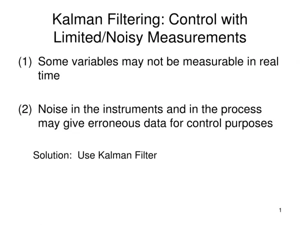
Kalman Filtering: Control with Limited/Noisy Measurements (1) Some variables may not be measurable in real time • Noise in the instruments and in the process may give erroneous data for control purposes Solution: Use Kalman Filter
Random Variables Ex turbulent flow, temperature sensor in boiling liquid mean (expected) value of r.v. : expected value operator p(x) probability density function
variance, covariance for two random variables, x and y, the degree of their dependence is indicated by covariance
Correlation coefficient extension to multivariable case: covariance matrix
State Estimation Object: Using data (which is filtered), reconstruct values for unmeasured state variables Definitions: variance s2 large, lots of scatter! single data pt. is unreliable Example: 2 measurements of equal reliability data pt. “p” data pt. “r” (actually data vectors) more generally,
error vectors → error covariance matrices = Similarly,
Select F so that is a minimum (least squares estimate or minimum variance estimate) scalar example:
For dynamic systems, we have 2 sources of information: • (xp) (1) state equation (and previous state estimates) • (xr) (2) new measurements at time step k • (but # measurements < # states) • x (k) = A (k-1) x (k-1) + G (k-1) w (k-1) • linear dynamic system; w = process noise • state variables xnx1
y: measured variables We wish to update (the estimates of the states) from inaccurate or unknown initial conditions on x(k), measurements corrupted by noise. The Kalman filter eqn: difference between measurement and estimate n.b. if we can’t measure xi (k), then xi(0) is unknown
Define covariance matrices process noise vector (white) instrument noise vector (white) Q, R usually diagonal matrices that can be “tuned” (variances needed) w, v are uncorrelated white noises (characteristics defined by mean, variance) markov sequence p(w(k+1) / w(k)) = p(w(k+1)) define state error covariance x: true value State estimate covariance
given an unbiased estimate (min. variance) is covariance matrix: = (1)
Inverting, estimate Ex C = [ 1 0 ] select D = [ 0 1 ] to make H1 invertible R = 1 potential for roundoff error
Combine xrand xp to minimize variance actually,
examine covariance of composite estimate becomes nxn matrix inverse By rearrangement and matrix identity (reduce size of inverse to be computed)
Summary of Recurrence Relations (1) (2) (3) (4) : Kalman gain matrix
Algorithm (1) (2) (3) (4) update return to (1),(2) to generate P(2), K(2) n.b. If A, G are not functions of k, P(k), K(k) can be generated ahead of time.
Extensions Kalman filter becomes
Properties of Kalman Filter (a) It provides an unbiased estimate (b) P(t) is the covariance matrix of P(t) found by soln of Riccati eqn. and does not depend on y(t) – can be calculated a priori (variance) note that
(c) Kalman filter is a linear, minimum variance estimator linear o.d.e. relating For non-white (colored) noise, optimal estimator is not necessarily linear (d) For long times s.s. Riccati eqn. don’t have to update gain matrix • (e) note similarity to LQP) • (Kalman filter uses initial condition)
Extension of K.F. to nonlinear systems (involves • successive linearization of state eqn.) • (g) Q,R. difficult to estimate a priori, but can be used • as design parameters • (relative values of Q, R are important) (h) (implies process noise is large) large R (small Q) small K (implies measurement noise is large)