Aggregate Equilibrium
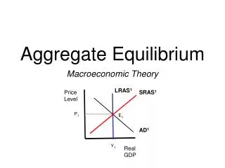
Aggregate Equilibrium. Macroeconomic Theory. Recessionary Gap. Economy above full output. LRAS 1. LRAS 1. Price Level. Price Level. SRAS 1. SRAS 1. Real GDP. Real GDP. AD 1. AD 1. Inflationary Gap. Economy below full output. Unemployment high, output low

Aggregate Equilibrium
E N D
Presentation Transcript
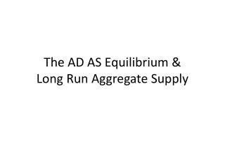
Aggregate Equilibrium Macroeconomic Theory
Recessionary Gap Economy above full output LRAS1 LRAS1 Price Level Price Level SRAS1 SRAS1 Real GDP Real GDP AD1 AD1 Inflationary Gap Economy below full output Unemployment high, output low Below PPF, Actual Px level < Expected Unemployment very low, output high Above PPF, Actual Px level > Expected
Short Run vs. Long Run • In short run, a shift in AD cause changes in real GDP, Unemployment & price level • In long run, wages & prices are not “sticky” and do not affect output • Prices are perfectly flexible in long run • Actual price level must equal expected price level
LONG RUN EQUILIBRIUM IN LONG RUN EQUILIBRIUM: This must be true: Expected Price Level = Actual Price Level Employment = Full Employment Real GDP = Potential Output Quantity = Natural rate + a( Actual Px - Expected Px) Supplied of Output ( Level Level )
2- causes output to fall in short run . . . SRAS1 SRAS2 3. . . . but over time, the SRAS A Shifts as expected Price level falls P . . B P2 1-Decrease in AD P3 C AD1 AD2 Y2 Y 4. . . . and output returns to its natural rate. Example: Stock Market Crash Short run —Step 1 & 2 Price Long Run– Step 3 & 4 Level LRAS . Real GDP 0
Analyzing Economic Changes • Four step process: • (1)Determine if the event affects SRAS, LRAS or AD • (2) Decide which direction curve shifts • (3) Compare the initial & new equilibrium • (4) Determine both short & long run equilibrium
Stagflation • A period of recession and inflation. • Output falls & price level rises • Example: late 1970’s in USA (oil crisis) • Challenge:Policymakers who can influence aggregate demand cannot offset both simultaneously
“Supply Shock” in SRAS • Consider an adverse shift in short run aggregate supply: • curve shifts to the left • Output falls below natural rate of employment • BOTH unemployment & price level rise
1. An adverse shift in SRAS (supply shock). SRAS2 B P2 A P 3. . . . and the price level to rise. AD Y2 Y 2. . . . causes output to fall . . . Example:“Supply Shock” Price Level LRAS SRAS1 Quantity of 0 Output