Download
1 / 41
430 likes | 488 Views
Exploring factors determining GDP, causes of inflation & unemployment. Concepts of aggregate output, income, consumption, and saving in macroeconomics.

E N D
The Core of Macroeconomic Theory This chapter starts presenting macroeconomic theory. 1. What factors determine GDP? 2. What causes inflation and unemployment? B. Macroeconomics divides the economy into three sectors: 1. Newly-produced goods and services (GDP) markets 2. Assets markets (financial and real) 3. Labor markets
Aggregate Output andAggregate Income (Y) • Aggregate output is the total quantity of goods and services produced (or supplied) in an economy in a given period. • Aggregate income is the total income received by all factors of production in a given period • When aggregate output increases, additional income is generated and vice versa.
Aggregate Output andAggregate Income (Y) • Aggregate output (income) (Y) is a combined term used to remind you of the exact equality between aggregate output and aggregate income. • When we talk about output (Y), we mean real output, or the quantities of goods and services produced, not the dollars in circulation.
Income, Consumption,and Saving (Y, C, and S) • A household can do two, and only two, things with its income: It can buy goods and services—that is, it can consume—or it can save. • Saving (S) is the part of its income that a household does not consume in a given period. Distinguished from savings, which is the current stock of accumulated saving. • The triple equal sign means this is an identity, or something that is always true.
Explaining Spending Behavior • All income is either spent on consumption or saved in an economy in which there are no taxes. Saving / Aggregate Income - Consumption
Household Consumption and Saving • Some determinants of aggregate consumption include: • Household income • Household wealth • Interest rates • Households’ expectations about the future • In The General Theory, Keynes argued that household consumption is directly related to its income.
Household Consumption and Saving • The relationship between consumption and income is called the consumption function. • For an individual household, the consumption function shows the level of consumption at each level of household income.
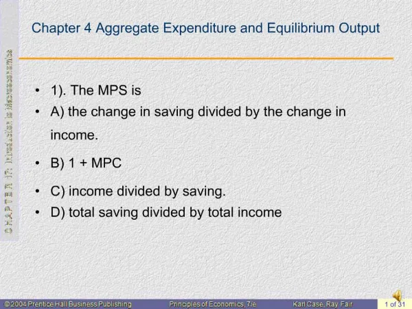
Household Consumption and Saving • The slope of the consumption function (b) is called the marginal propensity to consume (MPC), or the fraction of a change in income that is consumed, or spent.
Household Consumption and Saving • The fraction of a change in income that is saved is called the marginal propensity to save (MPS). • Once we know how much consumption will result from a given level of income, we know how much saving there will be. Therefore,
An Aggregate Consumption FunctionDerived from the Equation C = 100 + .75Y
An Aggregate Consumption FunctionDerived from the Equation C = 100 + .75Y • At a national income of zero, consumption is $100 billion (a). • For every $100 billion increase in income (DY), consumption rises by $75 billion (DC).
Because S = Y – C, it is easy to derive a saving function from a consumption function. A 45° line drawn from the origin can be used as a convenient tool to compare consumption and income graphically. • At Y = 200, consumption is 250. The 45° line shows us that consumption is larger than income by 50. Thus S =Y – C = 250. At Y = 800, consumption is less than income by 100. Thus, S = 100 when Y = 800.
The consumption function and the saving function are mirror images of one another. No information appears in one that does not also appear in the other. • These functions tell us how households in the aggregate will divide income between consumption spending and saving at every possible income level. In other words, they embody aggregate household behavior.
Planned Investment (I) • Consumption, as we have seen, is the spending by households on goods and services, but what kind of spending do firms engage in? The answer is investment. • Investment refers to purchases by firms of new buildings and equipment and additions to inventories, all of which add to firms’ capital stock. • To an economist, an investment is something produced that is used to create value in the future.
Spending on buildings and equipment is called business fixed investment. • inventories are part of the capital stock. When firms add to their inventories, they are investing—they are buying something that creates value in the future • One component of investment— is inventory change—is partly determined by how much households decide to buy, which is not under the complete control of firms. • change in inventory = production – sales
Actual versus Planned Investment • Desired or planned investment refers to the additions to capital stock and inventory that are planned by firms. • Because we assume households have complete control over their consumption, planned consumption is always equal to actual consumption, while planned investment is not always equal to actual investment)
Actual Versus Planned Investment • A firm may not always end up investing the exact amount that it planned. • Actual investment, is the actual amount of investment that takes place. If actual inventory investment turns out to be higher than firms planned, then actual investment is greater than I, planned investment.
The Planned Investment Function I • For now, we will assume that planned investment is fixed. It does not change when income changes. • this means the planned investment function is a horizontal line.
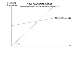
Planned Aggregate Expenditure (AE) • Planned aggregate expenditure is the total amount the economy plans to spend in a given period. It is equal to consumption plus planned investment.
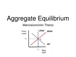
Equilibrium Aggregate Output (Income) • we have described the behavior of firms and households. We now discuss the nature of equilibrium and explain how the economy achieves equilibrium. • Equilibrium occurs when there is no tendency for change. In the macroeconomic goods market, equilibrium occurs when planned aggregate expenditure is equal to aggregate output. Planned AE = Planned Outputs
Equilibrium AggregateOutput (Income) aggregate output /Yplanned aggregate expenditure /AE/C + Iequilibrium: Y = AE, or Y = C + I Disequilibria: Y > C + I aggregate output > planned aggregate expenditureinventory investment is greater than plannedactual investment is greater than planned investment C + I > Yplanned aggregate expenditure > aggregate outputinventory investment is smaller than plannedactual investment is less than planned investment
(1) (2) (3) Equilibrium AggregateOutput (Income) There is only one value of Y for which this statement is true. We can find it by rearranging terms: By substituting (2) and (3) into (1) we get:
The Saving/InvestmentApproach to Equilibrium • Because aggregate income must either be saved or spent, by definition, Y= C + S, which is an identity. The equilibrium condition is Y = C + I, but this is not an identity because it does not hold when we are out of equilibrium. By substituting C + S for Y in the equilibrium condition, we can write:
The Saving/InvestmentApproach to Equilibrium • The saving/investment approach to equilibrium is C + S = C + I. Because we can subtract C from both sides of this equation, we are left with S = I. Thus, only when planned investment equals saving will there be equilibrium.
The Saving/InvestmentApproach to Equilibrium • saving is like a leakage out of the spending stream. Only if that leakage is counterbalanced by some other component of planned spending can the resulting planned aggregate expenditure equal aggregate output. This other component is planned investment (I).
The Saving/InvestmentApproach to Equilibrium • The leakage out of the spending stream—saving—is matched by an equal injection of planned investment spending into the spending stream. For this reason, the saving/investment approach to equilibrium is also called the leakages/injections approach to equilibrium.
The Saving/InvestmentApproach to Equilibrium If planned investment is exactly equal to saving, then planned aggregate expenditure is exactly equal to aggregate output, and there is equilibrium.
The S = I Approach to Equilibrium • Aggregate output will be equal to planned aggregate expenditure only when saving equals planned investment (S = I). Saving and planned investment are equal at Y=500.
The Multiplier • The multiplier is the ratio of the change in the equilibrium level of output to a change in some autonomous or independent variable. • An autonomous variable is a variable that is assumed not to depend on the state of the economy—that is, it does not change when the economy changes.
The Multiplier • In this chapter, for example, we consider planned investment to be autonomous. • The multiplier of autonomous investment describes the impact of an initial increase in planned investment on production, income, consumption spending, and equilibrium income.
The Multiplier • The size of the multiplier depends on the slope of the planned aggregate expenditure line.
The Multiplier • After an increase in planned investment, equilibrium output is four times the amount of the increase in planned investment.
The Size of the Multiplierin the Real World • The size of the multiplier in the U.S. economy is about 1.4. For example, a sustained increase in autonomous spending of $10 billion into the U.S. economy can be expected to raise real GDP over time by $14 billion.
The Paradox of Thrift • When households become concerned about the future and decide to save more, the corresponding decrease in consumption leads to a drop in spending and income. • Households end up consuming less, but they have not saved any more.
actual investment aggregate income aggregate output aggregate output (income) (Y) autonomous variable change in inventory consumption function desired, or planned, investment (I) equilibrium identity investment marginal propensity to consume (MPC) marginal propensity to save (MPS) multiplier paradox of thrift planned aggregate expenditure (AE) saving (S) Review Terms and Concepts