Download
1 / 44
440 likes | 627 Views
USING ROBUST PARAMETER DESIGN IN INDUSTRIAL EXPERIMENTS. William R. Myers Statistical Quality Control Section Biometrics and Statistical Sciences Department The Procter & Gamble Company BASS XI November 2, 2004. Robust Parameter Design History.

E N D
USING ROBUST PARAMETER DESIGN IN INDUSTRIAL EXPERIMENTS William R. Myers Statistical Quality Control Section Biometrics and Statistical Sciences Department The Procter & Gamble Company BASS XI November 2, 2004
Robust Parameter Design History • Genechi Taguchi: Japanese quality consultant (1950’s) • Introduced in the United States in 1980 • First Users: AT&T Bell Labs, Ford, ITT, Xerox among others • Statistical research and industrial application of Robust • Parameter Design have flourished since • Not extensively used in the Pharmaceutical Industry
Robust Parameter Design • Main emphasis is on variation reduction • A cost effective approach for reducing variation • Used to build quality into a new product/process or improve • quality of an existing one
Robust Parameter Design Diagram Output System Control Variables “Easy to Control” Noise Variables “Hard to Control” BASIC IDEA: Identify settings of control variables that dampen the effect of noise variables on the systems performance GOAL: Make the system Robustto variation in noise variables
Control Variables Those factors within a system that remain unchanged once their levels are selected • Examples • Speed • Pressure • Temperature • Mixing Time • Compression Force • Spray Rate
Noise Variables Those factors within a system that are difficult to control during normal process or design of a product (but can be controlled in an experimental situation) • Examples • Humidity • Moisture Content of Material • Consumer Use of a Product • Tolerance in the Control Variables • Variation in Raw Materials • Suppliers
Noise Variables The noise variable(s) is a random variable with an assumed distribution, e.g., N(0 , ) z
Graphical Description of a Robust Setting Response Low High Robust Setting Noise Variable High Low Control Variable
Graphical Description of Non-Robust Situation Response Low High Noise Variable High Low Control Variable
Effect Ordering Principle and Design Implications • control-by-noise interactions • control main effects • noise main effects • Control-by-control interactions • control-by-control-by-noise interactions • 3. Noise-by-noise interactions The choice of the experimental design is critical!
Terminology • Location Factors: Control factors that significantly affect the mean response • Dispersion Factors: Control factors that interact with a noise factor and therefore significantly affect the variability • Adjustment Factors: Location factors that are not dispersion factors
Two-Step Procedure for Analysis for Nominal-the-Best Problem • Select the levels of the dispersion factors to minimize dispersion • Select the levels of the adjustment factors to bring the location on target
Response Surface Model Important control-by-noise interaction are the control variables are the noise variables
Variance Response Model residual variance process variance transmitted by the noise variables Slope Interpretation Find levels of the control variables that make the following quantity equal (or close) to zero
A Simple Case y = tablet characteristic control variables = time force noise variable = particle size distribution (PSD) Response Surface Model y = 0+ 1time + 2force + PSD + time×PSD + Variance Response Model Varz[y(time,PSD)] = ( + time)2× Var(PSD) +
Summary of Simple Case • Select high level of time to minimize variation • Use force to bring the mean on target On Target with Minimum Variance!
Review Distributional Assumptions for Continuous Noise Variables • The variance-covariance matrix of z is known N(0, ) • Often assumed that the covariance between the noise variables • is zero Variance Response Model Assuming Cov(z1,z2)=0
Categorical Noise Variables • Noise variables can be categorical in nature • - suppliers • - brands of equipment • - operators • - production shifts • - production lines
The Distribution of a Categorical Noise Variables is Multinomial • Consider a single noise variable z with rz +1 categories for which • P(Category i) = pi
A Simple Case • One control factor • One noise factor with three categories With category 3 as the baseline:
Variance Response Model In the case of a categorical noise variable, the variance response model is fully specified as long as the pi values are known
More Intuitive Expression For The Variance Response Model Average Response over the Noise Variables Variance Response Model
Minimization of the Variance Response Model • Minimization of the Varz[y(x,z)] over the control • variable space will focus on the categories • that have a high probability of being present • - that have a mean response that is far from the • average response • Minimization of the Varz[y(x,z)] is accomplished by making • the mean response for each of the categories to be as close to • one another as possible (in the case when pi values are equal)
Robust Setting in the Case of a Categorical Noise Variable (Each supplier is used with equal frequency (p1 = p2 = p3 = 1/3) Robust Setting
Changing of Pi values • Robust settings may change with changes in the pi values • - customer may drop a supplier • - the amount a supplier is used may change
Supplier 2 is eliminated Robust Setting Be careful when interpreting interaction plots when the pi values are unequal
Impact of Continuous and Categorical Noise Variable Assumptions • The robust setting and overall process variance estimate • can be affected by the variance and covariance estimate • of the continuous noise variables • Fewer assumptions for the categorical noise variable • than for the continuous noise variable • - often assume that there is no correlation between • noise variables (which will not always apply)
Process Optimization and Robustness Experiment - Example • Product Development wants to develop optimum and robust • centerline conditions • Understand which variables are key levers in the process • Since more than one supplier will be used it is important to • develop centerline conditions that are robust to different • suppliers (supplier is considered a noise variable)
Specifics of Experiment • Study the effects of temperature, pressure and speed on the • response variable • - These three factors are considered control variables • Different suppliers will furnish the raw material • - The engineers do not want to have a unique set of • manufacturing conditions for each supplier • - The supplier is a categorical noise variable
Response, Control and Noise Variables • Key Response Variable • Variable Defect: Continuous Response • (LSL = 3.0 , target = 4.5 , USL = 5.4) • Control Variables • Temperature (193 °C - 230 °C ) • Pressure (2.2 bar – 3.2 bar) • Speed (32 cpm, 42 cpm, 50 cpm) • Noise Variable • Supplier (S1, S2, S3)
Design Considerations • Number of experimental conditions • Select a design that can efficiently estimate important factors • Linear effects • Interaction effects • Quadratic effects • A full Central Composite design was too costly (~81 runs) • An optimal design based on D-efficiency (37 runs)
Specifics of Designed Experiment • A 37-run computer-generated design (D-efficiency) • Combined array allows the estimation of • control main effects • noise main effects • control x control interaction effects • control quadratic effects • control x noise interactions
Term Estimate Std Error t Ratio Prob>|t| Intercept 6.6735 1.040 6.42 <.0001 Pressure (Bar) -0.6109 0.202 -3.03 0.0050 Speed (cpm) -0.0078 0.021 -0.36 0.7189 Supplier 1 -2.1110 1.297 -1.63 0.1140 Supplier 2 -2.2090 1.344 -1.64 0.1106 Supplier 1*Speed (cpm) 0.0645 0.031 2.07 0.0469 Supplier 2*Speed (cpm) 0.0805 0.032 2.54 0.0164 Model Estimates From Experiment
Interaction Plot of Speed and Supplier (Pressure = 3.2 Bar)
Summary of Experiment • Speed was set at 32 cpm in order to minimize the • process variance • In order to bring the mean response close to target (4.5), the • pressure adjustment factor should be set at 3.2 Bar • In this particular example the robust setting of 32 cpm • does not change when the pi values change
Conclusions For Categorical Noise Variables • Less assumptions made with categorical noise • variables than with continuous noise variables • In the case of categorical noise variables the variance • response model is fully specified as long as the pi • values are known
Conclusions For Categorical Noise Variables • Minimization of the over the control • variable space will focus on the categories • that have a high probability of being present • - that have a mean response that is far from the • average response • Robust settings may change with changes in the • pi values
Mixture-Process Variable Experiments with Noise Variables • Mixture experiments are commonly used in the pharmaceutical • industry (e.g., formulation) • In these experiments the mixture variables, which are • components of the formulation, cannot be adjusted • independently of one another • The proportion of the mixture components sum to 1 • The process variables are additional factors that can be • controlled independently of one another
Mixture-Process Variable Experiments with Noise Variables • The goal of such an experiment is to find the levels of the • mixture variables and the control variables that are robust to • variation in the noise variables, while simultaneously • providing an acceptable mean response value
Response Surface Model mixture model coefficients Interaction of mixture and noise variables Interaction of mixture and control variables Interaction of mixture, control and noise variables
Variance Response Model residual variance process variance transmitted by the noise variables Slope Interpretation Find levels of the process control variables and mixture variables that make the following quantity equal (or close) to zero
Conclusion • Robust Parameter Design is a very valuable quality • improvement tool for reducing process/product variation