Applications Statistical Quality Control
Systems Engineering Program. Department of Engineering Management, Information and Systems. EMIS 7370/5370 STAT 5340 : PROBABILITY AND STATISTICS FOR SCIENTISTS AND ENGINEERS. Applications Statistical Quality Control. Dr. Jerrell T. Stracener, SAE Fellow. Leadership in Engineering.

Applications Statistical Quality Control
E N D
Presentation Transcript
Systems Engineering Program Department of Engineering Management, Information and Systems EMIS 7370/5370 STAT 5340 : PROBABILITY AND STATISTICS FOR SCIENTISTS AND ENGINEERS Applications Statistical Quality Control Dr. Jerrell T. Stracener, SAE Fellow Leadership in Engineering
An Application of Probability & Statistics Statistical Quality Control Statistical Quality Control is an application of probabilitistic and statistical techniques to quality control
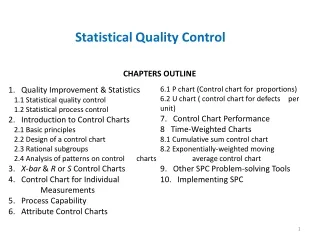
Statistical Quality Control - Elements Analysis of process capability Statistical process control Process improvement Acceptance sampling
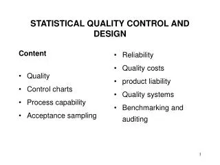
Statistical Tolerancing - Convention Normal Probability Distribution 0.00135 0.9973 0.00135 Nominal LTL UTL +3 -3
Statistical Tolerancing - Concept x LTL Nominal UTL
Caution For a normal distribution, the natural tolerance limits include 99.73% of the variable, or put another way, only 0.27% of the process output will fall outside the natural tolerance limits. Two points should be remembered: 1. 0.27% outside the natural tolerances sounds small, but this corresponds to 2700 nonconforming parts per million. 2. If the distribution of process output is non normal, then the percentage of output falling outside 3 may differ considerably from 0.27%.
Normal Distribution - Example The diameter of a metal shaft used in a disk-drive unit is normally distributed with mean 0.2508 inches and standard deviation 0.0005 inches. The specifications on the shaft have been established as 0.2500 0.0015 inches. We wish to determine what fraction of the shafts produced conform to specifications.
Normal Distribution - Example Solution f(x) 0.2500 nominal 0.2508 x 0.2485 LSL 0.2515 USL
Normal Distribution - Example Solution Thus, we would expect the process yield to be approximately 91.92%; that is, about 91.92% of the shafts produced conform to specifications. Note that almost all of the nonconforming shafts are too large, because the process mean is located very near to the upper specification limit. Suppose we can recenter the manufacturing process, perhaps by adjusting the machine, so that the process mean is exactly equal to the nominal value of 0.2500. Then we have
Normal Distribution - Example Solution f(x) nominal 0.2485 LSL 0.2515 USL x 0.2500
Using a normal probability distribution as a model for a quality characteristic with the specification limits at three standard deviations on either side of the mean. Now it turns out that in this situation the probability of producing a product within these specifications is 0.9973, which corresponds to 2700 parts per million (ppm) defective. This is referred to as three-sigma quality performance, and it actually sounds pretty good. However, suppose we have a product that consists of an assembly of 100 components or parts and all 100 parts must be non-defective for the product to function satisfactorily. Normal Distribution - Example
The probability that any specific unit of product is non-defective is 0.9973 x 0.9973 x . . . x 0.9973 = (0.9973)100 = 0.7631 That is, about 23.7% of the products produced under three sigma quality will be defective. This is not an acceptable situation, because many high technology products are made up of thousands of components. An automobile has about 200,000 components and an airplane has several million! Normal Distribution - Example