Download
1 / 42
430 likes | 603 Views
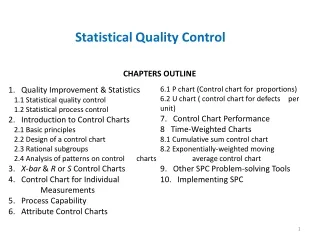
Statistical Quality Control Lab 202. By S. O. Duffuaa Systems Engineering Department. Salih Duffuaa.

E N D
Statistical Quality Control Lab 202 By S. O. Duffuaa Systems Engineering Department
Salih Duffuaa • Dr. Duffuaa is a Professor of Industrial and Systems Engineering at the Department of Systems Engineering at King Fahd University of Petroleum and Minerals, Dhahran, Saudi Arabia. He received his PhD in Operations Research from the University of Texas at Austin, USA. His research interests are in the areas of Operations research, Optimization, quality control, process improvement and maintenance engineering and management. He teaches course in the areas of Statistics, Quality control, Production and inventory control, Maintenance and reliability engineering and Operations Management. He consulted to industry on maintenance , quality control and facility planning. He authored a book on maintenance planning and control published by John Wiley and Sons and edited a book on maintenance optimization and control. He is the Editor of the Journal of Quality in Maintenance Engineering, published by Emerald in the United Kingdom.
King Fahd University of Petroleum & MineralsDepartment of Systems Engineering Errors and Test of Significance On November 17- 21, 2007
Objective of Session • Differentiate between Accuracy precision and bias. • Explain and measure precision and accuracy. • Identify and test outliers. • Formulate hypothesis about measured values. • Conduct simple significance tests.
Accuracy • Accuracy - The degree of agreement of a measured value with the true or expected value of the quantity of concern. Accuracy is measured by absolute error (E) or relative error Er • E = l Measured Value – True Value I. • Er = E/True value (100) percentage. • Measured value 10.2 , true value 10 • E = l 10.2 – 10.0 l = 0.2, Er = (0.2 /10) * 100 = 2%
Precision • Precision - The degree of mutual agreement characteristic of independent measurements as the result of repeated application of the process under specified condition. • Precision is the agreement between two or more measurements that have been made in exactly the same way. Precision is determined by replicating measurements. Precision can be measured by using the measures of dispersion:
Precision • Precision can be measured by using the measures of dispersion: • Range • Variance • Standard deviation • Coefficient of variation.
Precision ( Example) • Lab A made five measurements for the same property with the same instrument and procedures. The results are 9.80, 9.88, 10.02, 10.14, 10.21. • Mean = 10.01 • Standard deviation = 0.17 • Range = 0.41 • Variance = 0.0289 • COV = 1.72 % • E= .01. Er = 0.10%
Bias • Bias - A systematic error inherent in a method or caused by some artifact or idiosyncrasy or the measurement system. Bias may be both positive and negative, and several kinds can exist concurrently so that net bias is all that can be evaluated. • How to detect systematic errors?
Characteristic of A Measurement Process • Accuratewhen the value reported does not differ from the true value. • Biased when the error of the limiting mean is not zero, influenced by systematic error. • An accurate method is one capable of providing precise and unbiased results. In practice, we evaluate inaccuracy. Likewise, we evaluate imprecision, namely, the deviations of measurements.
Types of Errors • Random errors or chance errors are irregular and unpredictable. Random errors result in variability. In the determination of vanadium in crude, Ali has made six repeat determinations, and the results in ppm are: 20.2 19.9 20.1 20.4 20.2 20.4 • The determinations differ from each other because of random errors. If the test method did not introduce random error then the six determinations would be identical (assuming that gross errors are absent
Types Errors • Systematic errors: Determinate or systematic errors have a source that can usually be identified. They affect a sequence of determinations equally. They cause all the results from replicate measures to either be high or low. • Sources of systematic errors • Instrument • Methods • Operator or personal errors.
Types Errors • Gross errorsare defined as errors so serious that there may be no alternative but to make a completely new start, including new samples and lab tests. Examples of gross error include a complete instrument breakdown, power outage, loss or accidental discarding of data, and so on.
Problem 1 • Analyze the accuracy and precision of each of the following labs and identify which lab has a random systematic or gross errors. ( Explain if the lab is not precise or accurate how did you reach to the conclusion.
Example Page 4 Section 2 • Laboratory A— The random error is small because the measurements all go in one direction. The standard deviation and coefficient of variation are small, therefore the results are precise. Second, Lab A's results also include systematic error. Because all the results are in error in the same sense—too high. Systematic errors affect accuracy, or proximity to the true value. The error and relative error are high indicating a lack of accuracy. • Laboratory B—Laboratory B obtained an average 10.01. This result is in direct contrast to that of Lab. A. The average 10.01 is very close to our known true value of 10.00. We therefore can characterize the data as accurate and without substantial systematic error. However, the spread of the results is very large, indicating poor precision and the presence of substantial random error. • It should be noted that a comparison of Lab. A and Lab. B results clearly indicates that random and systematic errors can occur independently of each other.
Example Page 4 Section 2 • Laboratory C—Laboratory C's average of 9.90 and with a standard deviation of 0.21 and a coefficient of variation of 2.13%. The relative error is also high. This indicates that the data is neither precise nor accurate. • Laboratory D—Laboratory Dhas achieved an accurate mean and precise measures of dispersion and error.
Significance Tests/ Test of hypothesis • Purpose: To draw a conclusion about a population using data from a sample. • Test that the analytical procedure is not subject to systematic errors. • Test that the error is not significant. • Test that the population mean is equal to the sample mean. • Test that one lab results is more accurate than another lab.
Significance Tests/ Test of hypothesis • Test the precision of an instrument. • Compare the precision of two instruments. • Test that Arabs are taller than European.
Significance Tests/ Test of hypothesis • Significant tests are widely used in the evaluation of experimental results. In making a significance test we are testing the truth of a hypothesis, which is known as null hypothesis. • In all analytical procedures we adopt the null hypothesis that the analytical method employed is not subject to systematic error. The term null is used to imply that there is no difference between the observed and known values other than that which can be attributed to random variation
Significance Tests/ Test of hypothesis • Assuming that null hypothesis is true, statistical theory can be used to calculate the probability (i.e. the chance) that the observed difference between the sample mean and the true value μ, arises solely as a result of random error. • The lower the probability that the observed difference occurs by chance, the less likely it is that the null hypothesis is true. • Usually the null hypothesis is rejected if the probability of the observed difference occurring by chance is less than 1 in 20 (i.e. 0.05 or 5%) and in such a case the difference is said to be significant at the 0.05 (or 5%) level.
Demonstration • In this vanadium determination, it was believed that the true vanadium concentration was 20.1 ppm, but Mohammad's determinations had a mean of 20.7 ppm and a standard deviation of 0.179. Can we conclude Mohammed is biased?
One Sample t-test • Step 1: Null hypothesis – Mohammad is not biased (i.e his population mean μ is equal to 20.1). H0: = μ • Step 2: Alternative hypothesis – Mohammad is biased (i.e his population mean μ is not equal to 20.1). H1:≠μ
One Sample t-test • Step 3: Test statistic • Step 4: Critical values – from the t-table for a two sided test with 5 degree of freedom. 2.57 at the 5% significance level 4.03 at the 1% significance level • Step 5: Decision – We reject the null hypothesis. • Step 6: Conclusion – We concluded that Mohammad is biased.
Test Statistics When calculating the value of the t-test we took into account: • The deviation of the sample mean from the hypothesized population mean (μ). • The variability between repeat determinations that we would expect to find in the test method. This is quantified by the sample standard deviation. • The number of repeated determinations. • A large value of test statistic is an indication of bias. • In all significance tests, a large test statistic implies that the null hypothesis is false.
Hypothesis Testing • Hypothesis are suppositions, presumed to be true for subsequent testing. • Statistical significance is the level of probability selected to determine if a set of sample data is attributable to chance causes alone. • Chance causes are unknown factors that contribute to variation. They are generally numerous and individually of small magnitude. They are not readily detectable or identifiable
Alternative Way To test hypothesis • Example 15. Another example for large sample size • The strength specification of a filament is claimed to be 21.4 ounces. The strength of 120 filaments was randomly sampled. These are the results: • = 20.5 oz. • S = 1.1 oz. • n = 120 • Is the manufacturer's claim substantiated?
Alternative Way To test hypothesis • A common method of answering this question is to set up confidence limits for the mean. The confidence coefficient chosen was 95%. • From Equation 5: CL= ± 1.96(SEM) Therefore: • CL = 20.5 ± 1.96 20.5 ± 1.96 (0.10) = 20.5 ± 0.20 i.e. 20.30 to 20.70 ounces • The manufacturer's claim of 21.4 ounces is not within the 95% confidence limits for the mean of the sample. The claim seems to be incorrect on the basis of this batch of samples. We have just drawn a statistical inference on a population based on a sample.
Test of Significance • Ho = 21.4 • H1not =21.4 • = .05 • Test statistics Z = (X-bar - µ/ (/n) • Compute the value of test statistics and compare it to Z-table values • If Z-computes larger than table value reject null hypothesis.
Solution Example 18 • Step 1. Ho: = 0 H1: not = 0 • Step 2. Compare the pairs of values above, the differences are: Sample Difference 1 (71 - 76) = -5 2 (61 - 68) = -7 3 (50 - 48) = 2 4 (60 - 57) = 3 Mean of the difference, md, is
Solution Example 18 • t = = 0.7 • Compare this to table value with 3 degrees of freedom t-table 3.16 at .05 level of significance • Do not reject Ho.
Problem • It is suspected that an acid-base titrimetric method has a significant indicator error and thus tends to give results with a positive systematic error (i.e. positive bias). To test this, an exact 0.1M solution of acid is used to titrate 25.00 ml of an exactly 0.1M solution of alkali, with the following results. • 25.06 25.18 24.87 25.51 25.34 25.41 From this data we have: Mean = 25.228ml Standard deviation = 0.238 Test the hypothesis that the method has a bias.
Outliers ( Dixon Q ) • An outlier is one or more values that appear to differ markedly from the other values in the distribution. The presence of an outlier may distort the true value of a set of data. It therefore becomes necessary to identify outliers and determine whether they belong in the data distribution.
Example Outliers • Note: Dixon’s Q is calculated without regard to sign. • For example, the following values were obtained for nitrate concentration in four water samplings: • 0.403 0.410 0.401 0.380 • The last measurement (0.380) is suspect. Should it be rejected? We find out by first solving Dixon's Q at the 95% confidence level. • Dixon's Q was found to be 0.7.
Steps to Reject an outlier • Decide the probability level to set for rejection (5% is standard). • Consult the standard table of critical values (Table 17 & 35) to determine if our Q of 0.7 should be accepted or rejected. • The table of critical values lists for each sample size a corresponding critical value. If Q exceeds the critical value for the given sample size, then Q is rejected.