Statistical Quality Control

1. Statistical Quality Control

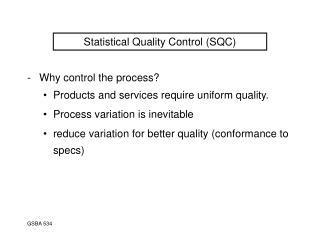
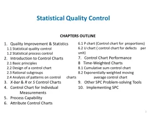
2. 15-1.2: Statistical Process Control • Statistical process control is a collection of tools that when used together can result in process stability and variance reduction

3. QMET – Quantitative Methods • Methods for dealing with quantitative data, not qualitative data. • Three ways to evaluate: • Normal distribution • Binomial distribution • Poisson distrribution

4. QMET – Quantitative Methods • Sample statistics are estimates of population parameters:

5. Normal Distribution

6. Normal Distribution Process: • Draw a diagram and label with given values i.e. μ (population mean), σ (population standard deviation and X (raw score) • Shade area required as per question • Convert raw score (X) to standard score (Z) using formula • Use tables to find probability: egp(0 < Z < z)

7. Normal Distribution Example Wool fibre breaking strengths are normally distributed with mean μ = 23.56 Newton and standard deviation, σ = 4.55. What proportion of fibres would have a breaking strength of 14.45 or less?

8. Normal Distribution Solution

9. Normal Distribution Solution

10. Normal Distribution Exercise The finish times for marathon runners during a race are normally distributed with a mean of 195 minute and a standard deviation of 25 minutes. • What is the probability that a runner will complete the marathon within 3 hours? • What proportion of the runners will complete the marathon between 3 hours and 4 hours?

11. Binomial Distribution • Applied to single variable discrete data where results are the numbers of “successful outcomes” in a given scenario. • no. of times the lights are red in 20 sets of traffic lights • No. of students with green eyes in a class of 40 • Used to calculate the probability of occurrences exactly, less than, more than, between given values

12. Binomial Distribution

13. Binomial Distribution Example: An automatic camera records the number of cars running a red light at an intersection (that is, the cars were going through when the red light was against the car). Analysis of the data shows that on average 15% of light changes record a car running a red light. Assume that the data has a binomial distribution. What is the probability that in 20 light changes there will be exactly three (3) cars running a red light?

14. Binomial Distribution Solution:

15. Binomial Distribution Exercise Executives in the New Zealand Forestry Industry claim that only 5% of all old sawmills sites contain soil residuals of dioxin (an additive previously used for anti-sap-stain treatment in wood) higher than the recommended level. If Environment Canterbury randomly selects 20 old saw mill sites for inspection, assuming that the executive claim is correct: • Calculate the probability that less than 1 site exceeds the recommended level of dioxin. • Calculate the probability that at most 2 sites exceed the recommended level of dioxin. • What is the probability that 1 or more of the 20 sites exceed the recommended level of dioxin?

16. Poisson Distribution • Known as the distribution of rare events • A Poisson process is where discrete events occur in a continuous, but finite interval of time or space.

17. Poisson Distribution • The following conditions must apply: • For a small interval the probability of the event occurring is proportional to the size of the interval • Events must not occur simultaneously • The interval is on some continuous measurement such as time, length or area • Each occurrence must be independent of others and must be at random • The events are often defects, accidents or unusual natural happenings, such as earthquakes, where in theory there is no upper limit on the number of events

18. Poisson Distribution • The parameter is λ (lambda). – average or mean number of occurrences over a given interval. • The probability function is:

19. Poisson Distribution Example: The average number of accidents at a level-crossing every year is 5. Calculate the probability that there are exactly 3 accidents there this year.

20. Poisson Distribution Exercise: A radioactive source emits 4 particles on average during a five-second period. • Calculate the probability that it emits 3 particles during a 5-second period • Calculate the probability that it emits at least one particle during a 5-second period • During a ten-second period, what is the probability that 6 particles are emitted?

21. Acceptance Sampling Plan Acceptance sampling – an inspection procedure used to determine whether to accept or reject a specific quantity of material. Basic procedure: • Take a random sample from a large quantity of items, test/measure it relative to the quality characteristic of interest • If the sample passes the test, the entire quantity of items is accepted • If the sample fail the test, either • The entire quantity of items is subjected to 100% inspection • The entire quantity is returned to the supplier

22. Sampling plans • Trying to keep the average number of items inspected (ANI) to a minimum • To keep the cost of inspection low. • Types of sampling plan: • Single-sampling plan • Double-sampling plan • Sequential-sampling plan

23. Single-sampling plan • A decision to accept or reject a lot based on the results of one random sample from the lot • Steps: • Take a random sample of size (n) and inspect each item • If the number of defects ≤ specified acceptance number (c), the consumer accept the entire lot • If the number of defects > c, the consumer subjects the entire lot to 100% inspection / reject the entire lot and returns it to the producer

24. Double-sampling plan • A plan in which management specifies two sample sizes (n1 & n2) and two acceptance numbers (c1 & c2): if the quality of the lot is very good or bad, the consumer can make a decision to accept or reject the lot on the basis of the first sample, which is smaller than the single-sampling plan.

25. Double-sampling plan • steps: • Take a random sample of size n1 • if number of defects ≤ c1, consumer accepts the lot • If number of defects > c2, consumer rejects the lot • If c1 ˂ number of defects ˂ c2, consumer takes a second sample of size n2 • If the combined number of defects in the two samples ≤ c2, consumer accepts the lot. Otherwise, it is rejected.

26. Sequential-sampling plan • A plan in which the consumer randomly selects items for the lot and inspects them one by one. • Each time an item is inspected, a decision is made • (1) reject the lot • (2) accept the lot • (3) continue sampling, based on the cumulative results

27. Sequential-sampling plan • Plots the total number of defectives against the cumulative sample size

28. Comparison of Sampling plans

29. Operating Characteristic Curves • Describe how well a sampling plan discriminates between good and bad lots. • shows probability of accepting lots of different quality levels for a specific sampling plan • Ideal OC curve can only be achieved with 100% inspection

30. X-axis shows % of items that are defective in a lot- “lot quality” Y-axis shows the probability or chance of accepting a lot As proportion of defects increases, the chance of accepting lot decreases Example: 90% chance of accepting a lot with 5% defectives; 10% chance of accepting a lot with 24% defectives Operating Characteristics (OC) Curves

31. Acceptable Quality Level (AQL) is the small % of defects that consumers are willing to accept; order of 1-2% Lot tolerance proportion defective (LTPD) is the upper limit of the percentage of defective items consumers are willing to tolerate Producer’s risk (α) is the chance a lot containing an acceptable quality level will be rejected; Type I error Consumer’s Risk (β) is the chance of accepting a lot that contains a greater number of defects than the LTPD limit; Type II error AQL, LTPD, Consumer’s Risk (α) & Producer’s Risk (β)

32. Producer’s and Consumer’s Risk (cont.) Accept Reject Type I Error Producer’ Risk Good Lot No Error Type II Error Consumer’s Risk Bad Lot No Error Sampling Errors

33. Operating Characteristic Curves (Example)

36. Operating Characteristic Curves (Example) Note that the plan provides a producer’s risk of 12.2% and a consumer’s risk of 12.6%. Both values are higher than the values usually acceptable for plans of this type (5 & 10%, respectively). Management can adjust the risks by changing the sample size.

37. Operating Characteristic Curves Sample size effect • Increasing n while holding c constant increases the producer’s risk and reduces the consumer’s risk.

38. Operating Characteristic Curves Acceptance level effect • Increasing c while holding n constant decreases the producer’s risk and increases the consumer’s risk

39. Operating Characteristic Curves (Exercise) A shipment of 2000 portable battery units for microcomputers is about to be inspected by a Malaysian importer. The Korean manufacturer and the importer have set up a sampling plan in which the α risk is limited to 5% at an acceptable quality level (AQL) of 2% defective, and the β risk is set to 10% at Lot tolerance percent defective (LTPD) = 7% defective. We want to construct the OC curve for the plan of n = 120 sample size and an acceptance level of c ≤ 3 defectives. Both firms want to know if this plan will satidfy their quality and risk requirements.

40. Operating Characteristic Curves (Solution) α = 1 – 0.779 = 0.221 or 22.1%, exceed the 5% level desired by the producer. β = 0.032 or 3.2%, well under the 10% sought by the consumer.

41. Operating Characteristic Curves (Solution)

42. 15-1.2: Statistical Process Control The eight major tools are 1) Histogram 2) Pareto Chart 4) Cause and Effect Diagram 5) Defect Concentration Diagram 6) Control Chart 7) Scatter Diagram 8) Check Sheet

43. 15-2: Introduction to Control Charts 15-2.1 Basic Principles • A process that is operating with only chance causes of variation present is said to be in statistical control. • A process that is operating in the presence of assignable causesis said to be out of control. • The eventual goal of SPC is the elimination of variability in the process.

44. 15-2: Introduction to Control Charts 15-2.1 Basic Principles A typical control chart has control limits set at values such that if the process is in control, nearly all points will lie within the upper control limit (UCL) and the lower control limit (LCL). Figure 15-1A typical control chart.

45. 15-2: Introduction to Control Charts 15-2.1 Basic Principles where k = distance of the control limit from the center line w = mean of some sample statistic, W. w= standard deviation of some statistic, W.

46. 15-2: Introduction to Control Charts 15-2.1 Basic Principles Popularity of control charts 1) Control charts are a proven technique for improving productivity. 2) Control charts are effective in defect prevention. 3) Control charts prevent unnecessary process adjustment. 4) Control charts provide diagnostic information. 5) Control charts provide information about process capability.

47. 15-2: Introduction to Control Charts 15-2.1 Basic Principles Types of control charts • Variables Control Charts • These charts are applied to data that follow a continuous distribution. • Attributes Control Charts • These charts are applied to data that follow a discrete distribution.

48. CONTROL CHARTS ·        Used to test if the process is in control ·        Used to see if significant changes have occurred in the process over time “Discrete Data Charts” or “pn-p charts” Inspection on lot or batch Note # good/defective # of parts inspected in the lot = n Fraction of defective in lot = p Number of defectives = pn “Indiscreet” or “Continuous Data Chart” or “X-R Chart” Measurement at time intervals Measurements compared - control over time. Examples: Length (mm) Volume (cc) Weight (gm) Power (kwh) Time (sec) Pressure (psi) Voltage (v)

49. - R CHART CONSTRUCTION Class Example In the manufacturing process for this example parts are being machined with a nominal diameter of 13 mm. Samples are taken at the following times of day: 6:00, 10:00, 14:00, 18:00 and 22:00, for 25 consecutive days. The diameter measurements from these samples are presented on the table in the next slide.