Download
1 / 39
390 likes | 515 Views
ANOTHER CLOSE ENCOUNTER: WHEN PAINLEVÉ I MEETS THE WAVE EQUATION. R. GLOWINSKI & A. QUAINI. INTRODUCTION

E N D
ANOTHER CLOSE ENCOUNTER:WHEN PAINLEVÉ I MEETS THEWAVE EQUATION R. GLOWINSKI & A. QUAINI
INTRODUCTION Few months ago, while cleaning my office desk, I found a 2010 issue of the Notices of the AMS mentioning a newly started PainlevéProject, this project being a cyber meeting point for those scientists interested by all aspects of the six transcendent Painlevé equations. Intrigued by such a project, I went to WIKIPEDIA where I learnt that the 6 Painlevé equations read as (with j = 1, 2, …, 6) Rjbeing a complex-valued rational function of its three arguments. In this lecture, we will focus on the 1st Painlevé equation (Painlevé I), namely:
If y(0) = 0 and (dy/dt)(0) = 0, the graph of the solution looks like (with explosion (blow-up) at t ≈ 2.5):
Despite the fact that the 6 Painlevé equations occur in many applications, from Mechanics and Physics in particular, it seems that that there is still much to do concerning their numerical solution. A recent contribution in that direction is: B. FORNBERG & J.A.C. WEIDEMAN, A numerical methodology for the Painlevéequations, J. Comp. Phys., 230(15), 2011, 5957-5973. Our goal here is more modest: it consists in investigating the numerical solution of the following nonlinear wave equation, where Is aboundeddomain of R2:
and to study the dependence of the solutions with respect to cand the boundary conditions. Paul Painlevé(1863-1933)was twice France Prime Minister (it is reasonable to assume that Painlevéwent to Politics because Mathematics were too easy for him*, the same way that J. Von Neumann went to Physics, since, according to P. Lax, Mathematics were also too easy for him). It is worth mentioning that ‘the’ Emile Borelwas Secretary of the Navy in both Painlevé “cabinets ministeriels”, a most important information since J.L. Lions, and therefore his many PhD students (several of them are attending this conference), are E. Borel descendants (as are their own PhD students).
2. RELATED PROBLEMS In the Chapter I of his celebrated 1969 book “QuelquesMéthodes de Résolution des Problèmes aux Limites Non Linéaires”, J.L. Lions presents existence and non-existence results from D. Sattinger, J.B. Keller & H. Fujita concerning the solutions of the following nonlinear wave equation Concerning the solution of nonlinear parabolic equations with blow-up let us mention
A.A. SAMARSKII, V.A. GALAKTIONOV, S.P. KURDYUMOV & A.P. MIKHAILOV,Blow-Up in Quasi-Linear Parabolic Equations,1995 3. An operator-splitting approach to the numerical solution of the Painlevé I – Wave Equation problem The problem under consideration being ‘multi-physics’ (reaction-propagation type) and multi-time scales, an obvious candidate for its time discretization is the Strang’s Symmetrized Operator-Splitting Scheme (SSOS Scheme), that scheme being a reasonable compromise between simplicity, robustness and accuracy (more sophisticated, but more complicated, O.–S. schemes are available).In order to apply the SSOS scheme to the solution of our Painlevé I – Wave Equation problem, the 1ststep is to write the above problem as a 1st order in time PDE system. To do so, we introduce p = u/t, obtaining thus if we take u = 0 on (0, Tmax) as boundary condition:
With t > 0a time-discretizationstep, tn+ = (n+)t, and , (0, 1) with + = 1, we obtain by application of the SSOS scheme:
(1) u0 = u0 , p0 = u1. For n 0, {un, pn}{un+1, pn+1} via (2.1) {un+1/2, pn+1/2} = {u(tn+1/2), p(tn+1/2)}, {u, p} being the solution of (2.2)
(3.1) {u, p} being the solution of (3.2)
(4.1) {u, p} being the solution of (4.2) By (partial) elimination of p, we obtain the following O.S. scheme:
(5) u0 = u0 , p0 = u1. For n 0, {un, pn}{un+1, pn+1} via (6.1) ubeing the solution of (6.2)
(7.1) with u the solution of (7.2)
(8.1) ubeing the solution of (8.2)
4. On the solution of the linear wave-suproblems At each time-step, we have to solve a linear wave problem of the following type: (LWE) We assume that 0 H10(Ω) and 1 L2(Ω). A variational formulation of (LWE), well-suited to finite element implementation,is given by(LWE-V):
where < . , . > denotes theduality pairing between H – 1(Ω) and H10(Ω). Next, assuming that Ωis a boundedpolygonal sub-domain of R2, we introduce a triangulationThof Ωand the following finitedimensional finite element approximationof the space H10(Ω):
P1 being the space of the two variable polynomials of degree ≤ 1. We approximate (LWE-V) by (LWE-V)h defined as follows: with 0h and 1h both belonging to Vhand approximating 0and1, respectively.
Let us denote by Nh the set of the interior vertices Pjof Th (we have Nh= dim Vh) and by h(t) the Nh– dimensional vector We have then Above, the mass matrix Mhand the stiffness matrix Ahare both symmetric and positive definite. Now, let Q be a positive integer and define τby
For the time-discretization, we advocate the following non-dissipative second order accurate centered scheme(the subscripts h have been omitted): The stability condition of the above scheme is given by where N is the largest eigenvalue ofM –1A ( = O(h–2) here).
5. On the solution of the nonlinear suproblems At each time step of the Strang symmetrized scheme and for every vertex of Thwe have to solve two initial value problems of the following type: (NLOD2) Let M be a positive integer; we denote (tf – t0)/Mby and t0 + mby tm. We approximate then (NLOD2) by
The above scheme can be obtained by limiting to the second order the following Taylor expansion (TE)m
We can use the 3rd order term in (TE)mto adapt by observing that We advocate then the following adaptation strategy: (i) If keep integrating with (a typical value oftolbeing 10 – 4 ).
(ii) If the above inequality is not verified, divideby 2, as many times as necessary to have the above error estimator less than 0.2 tol. 6. NUMERICAL EXPERIMENTS All with Ω = (0, 1)2, Δx1 = Δx2 = 1/100 and 1/150, c Δt ≈ ½ Δx, Q = 3, and M = 3 (initially), α= β = ½. Initial conditions: u0 = 0, u1= 0. 6.1. Dirichlet Boundary conditions Roughly speaking, the blow up time is of the order of c2 (we stopped computing as soon as the max of the approximate solution reached 104). The results for both space discretization steps are essentially identical.
6.2. Dirichlet-SommerfeldBoundary conditions Consider Γ1= {{x1, x2}| x1 = 1, 0 < x2 < 1}, Γ0 = ∂Ω\Γ1 and take as boundary conditions For the same value of c the blow-up time is shorter than for pure homogeneous Dirichlet boundary conditions.
I don’t want to be polemical but I think that monolithic(un-split) schemes will have troubles at handling this nonlinear wave problem. By the way the approach discussed here is highly parallelizable. Thank you for your attention