Close Range Photogrammetry
Close Range Photogrammetry. Saju John Mathew EE 5358 Monday, 24 th March 2008 University of Texas at Arlington. Overview. Definitions Equipment Mathematical Explanations Working Applications. Close Range Photogrammetry(CRP).

Close Range Photogrammetry
E N D
Presentation Transcript
Close Range Photogrammetry Saju John Mathew EE 5358 Monday, 24th March 2008 University of Texas at Arlington EE 5358 Computer Vision
Overview • Definitions • Equipment • Mathematical Explanations • Working • Applications EE 5358 Computer Vision
Close Range Photogrammetry(CRP) • Photogrammetry is a measurement technique where the coordinates of the points in 3D of an object are calculated by the measurements made in two photographic images(or more) taken starting from different positions. • CRP is generally used in conjunction with object to camera distances of not more than 300 meters (984 feet). EE 5358 Computer Vision
Vertical Aerial Photographs University of Texas at Arlington at approx. 30 meters University of Texas at Arlington at approx. 200 meters EE 5358 Computer Vision
CRP It can be broadly divided into two main parts: • Acquiring data from the object to be measured by taking the necessary photographs. • Reducing the photographs (perspective projection) into maps or spatial coordinates (orthogonal projection). EE 5358 Computer Vision
Acquisition of Data: Camera Cameras can be broadly classified into two: • Metric • Single Cameras • Stereometric Cameras • Non-metric EE 5358 Computer Vision
Metric Cameras Photogrammetric Camera that enables geometrically accurate reconstruction of the optical model of the object scene from its stereo photographs Single Cameras • Total depth of field • Photographic material • Nominal focal length • Format of photographic material • Tilt range of camera axis and number of intermediate stops EE 5358 Computer Vision
Metric Cameras (contd.) Stereometric Cameras • Base Length • Nominal Focal Length • Operational Range • Photographic Material • Format of photographic material • Tilt range of optical axes and number of intermediate tilt stops EE 5358 Computer Vision
Non-metric Cameras Cameras that have not been designed especially for photogrammetric purposes: • A camera whose interior orientation is completely or partially unknown and frequently unstable. EE 5358 Computer Vision
Non-metric Cameras Advantages • General availability • Flexibility in focusing range • Price is considerably less than for metric cameras • Can be hand-held and thereby oriented in any direction Disadvantages • Lenses are designed for high resolution at the expense of high distortion • Instability of interior orientation (changes after every exposure) • Lack of fiducial marks • Absence of level bubbles and orientation provisions precludes the determination of exterior orientation before exposure EE 5358 Computer Vision
Data Reduction • Analog 1900 to 1960 • Analytical 1960 onwards • Semi-analytical • Digital 1980 onwards EE 5358 Computer Vision
Analytical Photogrammetry • Based on camera parameters, measured photo coordinates and ground control • Accounts for any tilts that exist in photos • Solves complex systems of redundant equations by implementing least squares method EE 5358 Computer Vision
Review L y Z f xa Collinearity Condition The exposure station of a photograph, an object point and its photo image all lie along a straight line. a Tilted photo plane ya x O Y ZL A Za Xa XL Ya YL X EE 5358 Computer Vision
Image Coordinate System z’ y’ • Ground Coordinate System - X, Y, Z wrt Ground Coordinate System • Exposure Station Coordinates – XL, YL, ZL • Object Point (A) Coordinates – Xa, Ya, Za • Rotated coordinate system parallel to ground coordinate system (XYZ) – x’, y’, z’ wrt Rotated Coordinate System • Rotated image coordinates – xa’, ya’, za’ • xa’ , ya’ and za’ are related to the measured photo coordinates xa, ya, focal length (f) and the three rotation angles omega, phi and kappa. L Z x’ za’ ya’ Xa’ ZL Y A Za Xa Ya XL YL X EE 5358 Computer Vision
Rotation Formulas • Developed in a sequence of three independent two-dimensional rotations. • ω rotation about x’ axis x1 = x’ y1 = y’Cosω + z’Sinω z1 = -y’Sinω + z’Cosω • φ rotation about y’ axis x2 = -z1Sinφ + x1Cosφ y2 = y1 z2 = z1Cosφ + x1Sinφ • κ rotation about z’ axis x = x2Cosκ + y2Sin κ y = -x2Sinκ + y2Cosκ z = z2 EE 5358 Computer Vision
Rotation Matrix X = MX’ Rotation Matrix The sum of the squares of the three “direction cosines” in any row or in any column is unity. M -1 = MT X’ = MTX x = x’(CosφCosκ) + y’(SinωSinφCosκ + CosωSinκ) + z’(-CosωSinφCosκ + SinωSinκ) y = x’(-CosφSinκ) + y’(-SinωSinφSinκ + CosωCosκ) + z’(CosωSinφSinκ + SinωCosκ ) z = x’(Sinφ) + y’(-SinωCosφ) + z’(CosωCosφ) x = m11x’ + m12y’ + m13z’ y = m21x’ + m22y’ + m23z’ z = m31x’ + m32y’ + m33z’ EE 5358 Computer Vision
Collinearity Condition Equations Collinearity condition equations developed from similar triangles * Dividing xa and ya by za * Substitute –f for za * Correcting the offset of Principal point (xo, yo) x = m11x’ + m12y’ + m13z’ y = m21x’ + m22y’ + m23z’ z = m31x’ + m32y’ + m33z’ EE 5358 Computer Vision
Collinearity Equations • Nonlinear • Nine unknowns • ω, φ, κ • XA, YA and ZA • XL, YL and ZL Taylor’s Theorem is used to linearize the nonlinear equations substituting EE 5358 Computer Vision
Linearizing Collinearity Equations Rewriting the Collinearity Equations • F0 and G0 are functions F and G evaluated at the initial approximations for the nine unknowns • dω, dφ, dκ are the unknown corrections to be applied to the initial approximations • The rest of the terms are the partial derivatives of F and G wrt to their respective unknowns at the initial approximations Taylor’s Theorem EE 5358 Computer Vision
Applying LLSM to Collinearity Equations • Residual terms must be included in order to make the equations consistent J = xa – Fo ; K = ya – Go b terms are coefficients equal to the partial derivatives Numerical values for these coefficient terms are obtained by using initial approximations for the unknowns. The terms must be solved iteratively (computed corrections are added to the initial approximations to obtain revised approximations) until the magnitudes of corrections to initial approximations become negligible. EE 5358 Computer Vision
Analytical Stereomodel • Mathematical calculation of three-dimensional ground coordinates of points in the stereomodel by analytical photogrammetric techniques • Three steps involved in forming an Analytical Stereomodel: • Interior Orientation • Relative Orientation • Absolute Orientation EE 5358 Computer Vision
Analytical Interior Orientation • Requires camera calibration information and quantification of the effects of atmospheric refraction. • 2D coordinate transformation is used to relate the comparator coordinates to the fiducial coordinate system to correct film distortion. • Lens distortion and principal-point information from camera calibration are used to refine the coordinates so that they are correctly related to the principal point and free from lens distortion. • Atmospheric refraction corrections are applied. EE 5358 Computer Vision
Analytical Relative Orientation • Process of determining the elements of exterior orientation • Fix the exterior orientation elements of the left photo of the stereopair to zero values • Common method in use to find these elements is through Space Resection by Collinearity(see slide below) • Each object point in the stereomodel contributes 4 equations • 5 unknown orientation elements + 3 unknowns(X, Y & Z) EE 5358 Computer Vision
Space Resection by Collinearity • Formulate the collinearity equations for a number of control points whose X, Y and Z ground coordinates are known and whose images appear in the tilted photo. The equations are then solved for the six unknown elements of exterior orientation which appear in them. Space Resection collinearity equations for a point A A two dimensional conformal coordinate transformation is used X = ax’ – by’ + Tx X, Y – ground control coordinates for the point Y = ay’ + bx’ + Ty x’, y’ – ground coordinates from a verticalphotograph a, b, Tx, Ty – transformation parameters EE 5358 Computer Vision
Analytical Absolute Orientation • Utilizes a 3D conformal coordinate transformation • Requires a min. of 2 horizontal and 3 vertical control points • Stereomodel coordinates of control points are related to their 3D coordinates in a cartesian coordinate system • Coordinates of all stereomodel points in the ground system can be computed by applying the transformation parameters EE 5358 Computer Vision
Bundle Adjustment Adjust all photogrammetric measurements to ground control values in a single solution Unknown quantities • X, Y and Z object space coordinates of all object points • Exterior orientation parameters of all photographs Measurements • x and y photo coordinates of images of object points • X, Y and/or Z coordinates of ground control points • Direct observations of the exterior orientation parameters of the photographs EE 5358 Computer Vision
Bundle Adjustment-Observations • Photo Coordinates - Fundamental Photogrammetric Measurements made with a comparator or analytical plotter. According to accuracy and precision the coordinates are weighed • Control Points – determined through field survey • Exterior Orientation Parameters – especially helpful in understanding the angular attitude of a photograph Regardless of whether exterior orientation parameters were observed, a least squares solution is possible since the number of observations is always greater than the number of unknowns. xij, yij – measured photo coordinatesoftheimage of point j onphoto i related to fiducial axis system xo, yo– coordinates of principal points in fiducial axis system f - focal length/principal distance Xj, Yj, Zj– coordinates of point j in object space m11i, m12i, …….,m33i – rotation parameters for photo i XLi, YLi, ZLi– coordinates of incident nodal point of camera lens in object space EE 5358 Computer Vision
Bundle Adjustment - Weights • Photo coordinates σ02 – reference variance σxij2 , σyij2 – variances in xij and yij resp. σxijyij = σyijxij – covariance of xij and yij • Ground Control coordinates • σXj2, σYj2, σZj2 – variances in Xj00, Yj00, Zj00 resp. • σXjYj = σYjXj – covariance of Xj00 with Yj00 • σXjZj = σZjXj – covariance of Xj00 with Zj00 • σYjZj = σZjYj – covariance of Yj00 with Zj00 • Exterior Orientation Parameters EE 5358 Computer Vision
Direct Linear Transformation (DLT) • This method does not require fiducial marks and can be solved without supplying initial approximations for the parameters Collinearity equations along with the correction for lens distortion δx, δy – lens distortion fx – pd in the x directionfy – pd in the y direction Rearranging the above two equations EE 5358 Computer Vision
DLT(contd.) The resulting equations are solved iteratively using LSM • Advantages - No initial approximations are required for the unknowns. • Limitations • - Requirement of atleast six 3D object space control points - Lower accuracy of the solution as compared with a rigorous bundle adjustment EE 5358 Computer Vision
Analytical Self Calibration The equations take into account adjustment of the calibrated focal length, principal-point offsets and symmetric radial and decentering lens distortion. xa, ya – measured photo coordinates related to fiducials xo, yo – coordinates of the principal point = xa – xo where = ya - yo EE 5358 Computer Vision
Analytical Self Calibration(contd.) k1, k2, k3 = symmetric radial lens distortion coefficients p1, p2, p3 = decentering distortion coefficients f = calibrated focal length r, s, q = collinearity equation terms Provides a calibration of the camera under original conditions which existed when the photographs were taken. Geometric Requirements - Numerous redundant photographs from multiple locations are required, with sufficient roll diversity - Many well-distributed image points be measured over the entire format to determine lens distortion parameters The numerical stability of analytical self calibration is of serious concern. EE 5358 Computer Vision
Applications • Automobile Construction • Machine Construction, Metalworking, Quality Control • Mining Engineering • Objects in Motion • Shipbuilding • Structures and Buildings • Traffic Engineering • Biostereometrics EE 5358 Computer Vision
Biomedical Applications • Linear tape and caliper measurements of inherently irregular three-dimensional biological structures are inadequate for many purposes. • Subtle movements produced by breathing, pulsation of blood, and reflex correction for control of postural stability. • Short patient involvement times, avoids contact with the patient and thereby avoiding risk of deforming the area of interest and spreading infection. • All medical photogrammetric measurements require further interpretation and analysis to allow meaningful information to be given to the end-user. EE 5358 Computer Vision
Bibliography • Kamara, H.M. (1979). Handbook of Non-Topographic Photogrammetry, American Society of Photogrammetry. • Wolf , Paul R., Dewitt, Bon A. (2000). Elements of Photogrammetry, McGraw Hill. • Devarajan, Venkat and Chauhan, Kriti (Spring 2008). Lecture Notes: Mathematical Foundation of Photogrammetry, EE 5358 University of Texas at Arlington. • Karara, H.M. (1989). Non-Topographic Photogrammetry, American Society for Photogrammetry and Remote Sensing. • Mitchell, H.L. and Newton, I. (2002). Medical photogrammetric measurement: overview and prospects. ISPRS Journal of Photogrammetry & Remote Sensing, 56, 286-294. EE 5358 Computer Vision
Acknowledgments • Dr. Venkat Devarajan • Kriti Chauhan EE 5358 Computer Vision