Download
1 / 11
110 likes | 140 Views
Explore GRB spectral analysis techniques with SAE David Band software on Windows, covering GBM binned analysis with XSPEC, LAT binned analysis with XSPEC, and LAT unbinned analysis with likelihood. Learn to analyze data such as lightcurves, count maps, and spectra while performing joint fits for multi-detector data. Get familiar with necessary files and tools, including photon files, spacecraft files, and XML models, to carry out binned and unbinned analyses. Detailed documentation and installation guide ensure a smooth learning experience.

E N D
Demonstration of GRB Spectral Analysis with the SAE David Band (GSSC/JCA-UMBC)
Outline • Preliminaries • GBM Binned Analysis with XSPEC • LAT Binned Analysis with XSPEC • LAT Unbinned Analysis with Likelihood • Documentation
Preliminaries—Software • This demonstration uses the SAE installed on Windows. • Currently, to install the SAE on Windows the user downloads and runs an executable. The only additional user operation is adding a ‘short-cut’ to the desktop! • The short-cut opens a DOS window in which the SAE is run. • Cygwin need not be installed. • Other utilities are useful, such as fv, ds9, a file manager (e.g., Windows Explorer) and an editor. • XSPEC does not run in this Windows environment, but using HERA (invoked through the current version of fv) the user can run XSPEC remotely at GSFC (given an internet connection).
Preliminaries—Burst Knowledge • The SAE does not provide tools to detect bursts, or determine their location, duration or time of occurrence (but see below). • The GBM and LAT will have onboard triggers, and a burst trigger will be part of the LAT quick-look pipeline. Positions and times will be distributed through GCN. Thus we assume that the user brings this information to the analysis. • But the analysis can be aided by looking at the GBM and LAT lightcurves, and the LAT count map. • In this demonstration the burst data are: • RA=57.54º • Dec=15.78º • Trigger (Mission Elapsed Time)=221142014. s • GBM emission 221142009-221142055 s
GBM Binned Analysis with XSPEC • Remember—the GBM consists of 12 NaI and 2 BGO detectors. The data from each detector are treated separately. • Necessary files: • Time-tagged events (TTE)—a list of GBM events from the time of the burst, by detector • Background file—a standard format PHA file specific to the burst and detector. Will be provided by GBM team, but user will have method to generate. • Response file—a standard format RSP file specific to the burst and detector. Will be provided by GBM team, but user will have tool to generate.
GBM Binned Analysis, cont. TTE File • Lightcurve: • Bin the TTE data using gtbin with ‘LC’ option. Result is a lightcurve FITS file. • Look at lightcurve FITS file with fv. Mission Elapsed Time can be converted to time relative to trigger. • Spectral analysis: • Bin the TTE data using gtbin with ‘PHA’ option. Result is a PHA file. This can be done for the TTE files from many detectors. • Fire up XSPEC. Read in PHA, background and response files. Fit spectrum. Joint fits to the spectra from many GBM detectors are possible. • Time for Demo gtbin Light curve file fv Light curve plot TTE File gtbin PHA file RSP and BAK File XSPEC Fit
LAT Binned Analysis with XSPEC • Necessary files: • Photon file (FT1). Extracted from GSSC server. • Spacecraft file (FT2, sometimes called pointing & livetime history file). Extracted from GSSC server. • Data exploration: • Refine data selection (position, time) by applying gtselect to photon file. Result is another photon file. • Look at location of photons using fv. • Create lightcurve using gtbin with ‘LC’ option. Result is lightcurve FITS file. • Look at lightcurve FITS file with fv. Mission Elapsed Time can be converted to time relative to trigger. • Iterate to refine data selection. Photon File gtselect Edited Photon File gtbin fv Light curve file fv Count map Light curve plot
LAT Binned Analysis, cont. • Spectral analysis: • Bin the photon data (after all selections) using gtbin with ‘PHA’ option. Result is a PHA file. • Create RSP file using gtrspgen. • Fire up XSPEC. Read in PHA and RSP files. No background file is necessary. Fit spectrum. • Time for Demo Photon File gtselect Edited Photon File gtbin PHA file RSP File gtrspgen XSPEC Fit
Joint Fits • Most spectral analyses will involve joint fits. • Multiple GBM NaI detectors (10 keV-3 MeV) • GBM BGO detector (150 keV-30 MeV) • LAT • With event lists spectra can be binned by gtbin over multiple time bins resulting in PHAII files. • Spectra must be over the same time range. • File defining time bins created by gtbindef; gtbin can read resulting file. • XSPEC performs joint fits.
LAT Unbinned Analysis with Likelihood • Unbinned analysis is carried out using the general point source methodology with the likelihood tool. Analysis is simplified since there is one source and essentially no background. • Therefore only gtlikelihood is run! The • Necessary files: • Photon file resulting from spatial and temporal selection • Spacecraft file • XML file with preliminary burst model • Time for Demo Photon file Spacecraft file XML model file gtlikelihood Fit
Documentation • The tools and analysis methodology will be included in the SAE documentation. • Installation guide. Status: currently written for internal use • Analysis threads—examples of standard analyses. Status: currently threads exist for exploring the LAT data and XSPEC-type LAT, GBM and joint spectral fits. See: http://glast-ground.slac.stanford.edu/workbook/pages/sciTools_gbmGrbAnalysis/sciTools_gbmGrbAnalysis.htm • Cicerone—full manual describing the data, the tools and the analysis methodology. Status: only partially written. • Reference manual—each tool is described along with all inputs. Status: complete. For example: http://glast-ground.slac.stanford.edu/workbook/pages/sciTools_gtbin/sciTools_gtbin.htm