Download
1 / 43
430 likes | 578 Views
Tensor and Emission Tomography Problems on the Plane. A. L. Bukhgeim S. G. Kazantsev A. A. Bukhgeim Sobolev Institute of Mathematics Novosibirsk, RUSSIA. Overview. 1) Transmission tomography inversion formula on the basis of SVD of the Radon transform scalar, vector and tensor cases.

E N D
Tensor and Emission Tomography Problemson the Plane A. L. Bukhgeim S. G. Kazantsev A. A. Bukhgeim Sobolev Institute of Mathematics Novosibirsk, RUSSIA
Overview • 1) Transmission tomography • inversion formula • on the basis of SVD of the Radon transform • scalar, vector and tensor cases • 2) Emission tomography • the first explicit inversion formula • (A.L.Bukhgeim, S.G.Kazantsev, 1997) • recent results that follow from it • scalar and vector cases • 2D problems, in a unit disc on the plane • Isotropic case • Fan-beam scanning geometry
Helmholtz Decomposition = + = + Potential Part 2-D Vector Field Solenoidal Part
Vectorial Radon Transform Normal Flow Radon Transform
Vectorial Radon Transform Solenoidal Part of the Vector Field Normal Flow Radon Transform
Vectorial Radon Transform Solenoidal Part of the Vector Field Normal Flow Radon Transform Potential Part of the Vector Field
Tensorial Radon Transform Consider a unit disk on the plane: Covariant symmetric tensor field of rank m: Due to symmetry it has m+1 independent components. • By analogy with the vector case: • similar decomposition into the solenoidal and potential parts, • define tensorial Radon transform. Refer to: V. A.Sharafutdinov “Integral Geometry of Tensor Fields” Utrecht: VSP, 1994.
SVD of the Radon Transform SVD is one of the methods for solving ill-posed problems: Consider two Hilbert spaces: H with O.N.B and K with O.N.S. Singular value decomposition of an operator Then its generalized inverse operator will look like: - can be unbounded. - truncated SVD.
SVD of the Radon Transform The presence of a singular value decomposition allows to: • describe the image of the operator, • invert the operator, • estimate its level of incorrectness. The first SVD of the Radon transform for the parallel-beam geometry was derived by Herlitz in 1963 and Cormack in 1964 (scalar case only). BukhgeimA.A., KazantsevS.G. “Singular-value decomposition of the fan-beam Radon transform of tensor fields in a disc” // Preprint of Russian Academy of Sciences,Siberian Branch. No. 86.Novosibirsk: Institute of Mathematics Press, October 2001. 34 pages.
Singular Values Radon Transform Inverse Radon Transform Integration Operator Differentiation Operator
Transmission Tomography: Numerical Examples (Scalar Case) Compare with the talk of Emmanuel Candes ! reconstruction from 300 fan-projections; N=298 reconstruction from 512 noisy fan-projections; N=446 (noise level: 20%) reconstruction from 512 noisy fan-projections; N=382 (noise level: 20%) reconstruction from 512 noisy fan-projections; N=318 (noise level: 20%) reconstruction from 512 noisy fan-projections; N=254 (noise level: 20%) reconstruction from 512 noisy fan-projections; N=510 (noise level: 20%) original image
Transmission Tomography: Numerical Examples (Scalar Case) reconstruction from 2048 noisy fan-projections; N=2046 (noise level: 5% in L2-norm) reconstruction from 2048 noisy fan-projections; N=1022 (noise level: 5% in L2-norm) reconstruction from 2048 noisy fan-projections; N=510 (noise level: 5% in L2-norm) reconstruction from 8 fan-projections; N=6 reconstruction from 16 fan-projections; N=14 reconstruction from 32 fan-projections; N=30 reconstruction from 64 fan-projections; N=62 reconstruction from 128 fan-projections; N=126 reconstruction from 256 fan-projections; N=254 reconstruction from 512 fan-projections; N=510 reconstruction from 1024 fan-projections; N=1022 original image
Transmission Tomography: Numerical Examples (Vector Case) original (solenoidal) vector field reconstruction from noisy (3%) projections reconstruction from non-uniform projections
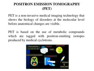
Emission Tomography AttenuatedRadon Transform • Assume, that the attenuation map of the object is known • Inject a radioactive solution into the patient, it is then spread all over the body with the blood • Place detectors around and measure how many radioactive particles go through it in the given directions • Reconstruct the Emission Map
Formulation of the emission tomography problem Consider a unit disc on the plane: Let represent an attenuation map and represent an emission map, both given in The fan-beam Radon transform The fan-beam attenuated Radon transform Emission tomography problem: reconstruct from its known attenuated Radon transform provided that the attenuation map is known.
Attenuated Vectorial Radon Transform Attenuated Normal Flow Radon Transform
Servey of the Results in Emission Tomography SCALAR CASE: • 1980, O.J. Tretiak, C. Metz. The first inversion formula for emission tomography with constant attenuation. • 1997, A.L. Bukhgeim, S.G. Kazantsev.The first explicit inversion formula for emission tomography (in the fan-beam formulation) with arbitrary non-constant attenuation (based on the theory of A-analytic functions). • 2000, R.G. Novikov (and then F.Natterer in 2001). Inversion formula for emission tomography in the parallel-beam formulation which then was numerically implemented by L.A. Kunyansky in 2001. VECTOR CASE: • 1997, K. Stråhlén. Inversion formula for full reconstruction of a vector field from both Exponential Vectorial Radon Transform and Exponential Normal Flow Transform, attenuation coefficient is constant. • 2002, A.A. Bukhgeim, S.G. Kazantsev. Full reconstruction of a vector field only from its Attenuated Vectorial Radon Transform, arbitrary non-constant attenuation function is allowed.
Equivalence of the Inversion Formulae Angular Hilbert Transform Hilbert Transform
Inversion formula (vector case) • components of the vector field • being reconstructed, - a known attenuation function: • For the full reconstruction of a vector field it’s sufficient to know only one transform: either Vectorial Attenuated Radon Transform or the Normal Flow Attenuated Radon Transform; • Arbitrary non-constant attenuation is allowed.
Emission Tomography: Numerical Examples (Scalar Case) 360 degree Medium Attenuation No Noise
Emission Tomography: Numerical Examples (Scalar Case) 360 degree Medium Attenuation Large Noise
Emission Tomography: Numerical Examples (Scalar Case) 360 degree XXL Attenuation [6,14] No Noise
Emission Tomography: Numerical Examples (Scalar Case) 270 degree Medium Attenuation No Noise
Emission Tomography: Numerical Examples (Scalar Case) 180 degree Medium Attenuation No Noise
Emission Tomography: Numerical Examples (Scalar Case) 90 degree ! Medium Attenuation No Noise
Emission Tomography: Numerical Examples (Scalar Case) 180 degree Large Attenuation [4,7] No Noise
Emission Tomography: Numerical Examples (Scalar Case) 180 degree Large Attenuation [4,7] With Noise
Emission Tomography: Numerical Examples (Vector Case) Sinogram Original Vector Field Reconstruction from 128 fan-projections
Emission Tomography: Numerical Examples (Vector Case) Sinogram Original Vector Field Reconstruction from 256 fan-projections
Emission Tomography: Numerical Examples (Vector Case) Sinogram Original Vector Field Reconstruction from 512 fan-projections
Emission Tomography: Numerical Examples (Vector Case) Sinogram Original Vector Field Reconstruction from 256 fan-projections
Emission Tomography: Numerical Examples (Vector Case) Sinogram Original Vector Field Reconstruction from 256 fan-projections
Emission Tomography: Numerical Examples (Vector Case) Sinogram Original Vector Field Reconstruction from 256 fan-projections
Conclusion • 1) SVD of the Radon transform of tensor fields • description of the image of the operator, • inversion formula, • estimation of incorrectness of the inverse problem, • unified formula (for reconstruction of scalar, vector and tensor fieds), • numerical implementation; • 2) The very first inversion formula (by A.L.Bukhgeim, S.G. Kazantsev) • was re-derived • shows equivalence of the first inversion formula to the formulae obtained later by Novikov and Natterer, • yields a pathbreaking inversion formula for the vectorial attenuated Radon transfom, • numerical implementation.