Chapter 11 Monopoly and Monopsony

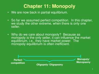
Chapter 11Monopoly and Monopsony Monopoly: one parrot.

Chapter 11 Outline Challenge: Pricing Apple’s iPad 11.1 Monopoly Profit Maximization 11.2 Market Power and Welfare 11.3 Taxes and Monopoly 11.4 Causes of Monopolies 11.5 Government Actions that Reduce Market Power 11.6 Monopoly Decisions Over Time and Behavioral Economics 11.7 Monopsony Challenge Solution

Challenge: Pricing Apple’s iPad • Background: • Apple started selling the iPad on April 3, 2010. • People loved the original iPad. Even at $499 for the basic model, Apple had a virtual monopoly on high-end tablets in its first year. The company still has a stronghold on the high-end tablet market. • Questions: • How did Apple set the price for the iPad when it was essentially the only game in town? (See Solved Problem 11.2) • How did the presence of me-too rival products produced by firms with higher marginal costs affect Apple’s pricing more recently? (See Challenge Solution)

11.1 Monopoly Profit Maximization • A monopoly is the only supplier of a good for which there is no close substitute. • Monopolies are not price takers like competitive firms • Monopoly output is the market output • Monopoly demand curve is the market demand curve • Monopolists can set their own price given market demand • Because demand is downward sloping, monopolists set price above marginal cost to maximize profit. • Like all firms, monopolies maximize profits by setting price or output so that marginal revenue (MR) equals marginal cost (MC).

11.1 Monopoly Profit Maximization • Monopolies maximize profits by setting price or output so that marginal revenue (MR) equals marginal cost (MC). • Profit function to be maximized by choosing output, Q: • (Q) = R(Q) – C(Q), where • R(Q) is the revenue function • C(Q) is the cost function • The necessary condition for profit maximization: • The sufficient condition for profit maximization:

11.1 Monopoly Profit Maximization • A firm’s MR curve depends on its demand curve. • MR is also downward sloping and lies below D • If p(Q) is the inverse demand function, which shows the price received for selling Q, then the marginal revenue function is: • Given a positive value of Q, MR lies below inverse demand. • Selling one more unit requires the monopolist to lower the price • Price is lowered on the marginal unit and all other units sold

11.1 Monopoly Profit Maximization • Moving from Q to Q+1, the monopoly’s marginal revenue is less than the price it charges by an amount equal to area C

11.1 MR Curve and the Price Elasticity of Demand • We can rewrite MR function so that it is stated in terms of elasticity: • This makes the relationship between MR, D, and elasticity quite clear. • Where demand hits the vertical axis, MR=P and demand is perfectly elastic. • Everywhere that MR > 0, demand is elastic. • The quantity at which MR = 0 corresponds to the unitary elastic portion of the demand curve. • Everywhere that MR < 0, demand is inelastic.

11.1 MR Curve and the Price Elasticity of Demand • Relationship for inverse demand function of and marginal revenue function of

11.1 Monopoly Example • Inverse demand function: • Can be used to find the marginal revenue function: • Quadratic SR cost function: • Can be used to find the marginal cost function: • Profit-maximizing output is obtained by producing Q*: • Solving this expression reveals Q*=6 • The inverse demand function indicates that people are willing to pay p = $18 for 6 units of output.

11.1 Monopoly Example • The monopolist’s profit maximizing choice of output is found where MR=MC. • At the profit-maximizing output, set p according to inverse demand.

11.1 Monopoly Example • Should a profit-maximizing monopoly produce at Q* or shut down? • As with competitive firms, a monopoly should shut down in the monopolist’s price is less than its AVC. • In our example, AVC at Q* of 6 is $6. • Because p = $18 is clearly above $6, the monopoly in this example should produce in the SR.

11.1 Effects of a Shift of Demand Curve • Shifts in demand that would affect the equilibrium output in a competitive market need not affect monopolist’s profit-maximizing output, Q*

11.2 Market Power and Welfare • Market power is the ability of a firm to charge a price above marginal cost and earn a positive profit. • Monopoly has market power; competitive firms do not. • Market power is related to the price elasticity of demand • Recall that • Rewrite as • Thus, the ratio of price to MC depends only on the elasticity of demand at the profit maximizing quantity. • The more elastic the demand curve, the less a monopoly can raise its price without losing sales (and vice versa).

11.2 Market Power • The Lerner Index (or price markup) is another way to examine the way in which elasticity affects a monopoly’s price relative to its MC. • The Lerner Index ranges from 0 to 1 for a profit-maximizing firm. • Competitive firms have a Lerner Index of 0. • The Lerner Index gets closer to 1 as a firm has more market power (and faces less elastic demand).

11.2 Sources of Market Power • Elasticity of the market demand curve depends on consumers’ tastes and options. • Demand becomes more elastic (which implies less market power for the firm): • as better substitutes for the firm’s product are introduced • as more firms enter the market selling a similar product • as firms that provide the same service locate closer to the firm • As a profit-maximizing monopoly faces more elastic demand, it has to lower its price. • Examples: Xerox, USPS, McDonald’s

11.2 Effects of Market Power on Welfare • Recall from Chapter 9 that competition maximizes welfare, which is the sum of consumer surplus and producer surplus, because price equals marginal cost. • By contrast, a monopoly • sets price above marginal cost (and above the competitive price) • causes consumers to buy less than the competitive level of output • generates deadweight loss

11.2 Effects of Market Power on Welfare • The competitive equilibrium, ec, has no DWL, while the monopoly equilibrium, em, has DWL = C+E.

11.3 Taxes and Monopoly • Taxes (ad valorem and specific) affect monopoly differently than a competitive industry: • Tax incidence on consumers (the change in the consumers’ price divided by the change in the tax) can exceed 100% in a monopoly market but not a competitive market. • If tax rates α and τ are set so that the after-tax output is the same with either type of tax, the government raises the same amount of tax revenue in a competitive market using either type of tax, but raises more revenue using an ad valorem tax than a specific tax under monopoly.

11.3 Taxes and Monopoly • Comparative Statics (of specific tax, τ) • Before-tax cost function is C(Q) • After-tax cost function is C(Q) + τQ • Necessary condition for maximizing after-tax profit: • Derivative (with respect to τ) of the sufficient condition for maximizing after-tax profit: • As the specific tax rises, the monopoly reduces its output. • Downward sloping means the monopoly raises its price.

11.3 Taxes and Monopoly • Tax Incidence on Consumers • Consumer price may rise by an amount greater than the tax. • Assume constant marginal cost, m, and inverse demand function with constant elasticity, ε, p = Q1/ε • Maximize profit by equating after-tax marginal cost and marginal revenue: • Substituting for Q in inverse demand yields the price set by monopoly: • Differential with respect to τ is greater than one because monopoly operates on elastic portion of demand curve.

11.3 Taxes and Monopoly • Governments typically use an ad valorem tax rather than a specific tax because the tax revenue is greater.

11.4 Causes of Monopolies • Why are some markets monopolized? • Two key reasons: • Cost advantage over other firms • Government created monopoly

11.4 Cost Advantages of Monopoly • Sources of cost advantages: 1. Control of an essential facility, a scarce resource that a rival firm needs to use to survive • Example: owning the only quarry in a region generates a cost advantage in the production of gravel 2. Use of superior technology or a better way of organizing production • Example: Henry Ford’s assembly lines and standardization 3. Protection from imitation through patents or informational secrets • Secrets are more common in new and improved processes; patents more common with new products

11.4 Cost Advantages of Monopoly • A market has a natural monopoly if one firm can produce the total output of the market at lower cost than several firms could. • where Q = q1 + q2 +…+ qn for n > 1 firms • Examples: public utilities such as water, gas, electric, and mail delivery • Natural monopolies may have high fixed costs, but low and fairly constant marginal costs.

11.4 Cost Advantages of Monopoly • A natural monopoly has economies of scale at all levels of output, so average costs fall as output increases.

11.5 Government Actions that Create Monopolies • Governments typically create monopolies in 1 of 3 ways: • By making it difficult for new firms to obtain a license to operate • Example: U.S. cities require new hospitals to secure a certificate of need to demonstrate the need for a new facility • By granting a firm the rights to be a monopoly • Example: public utilities operated by private company • By auctioning the rights to be a monopoly • Example: selling government monopolies to private firms (privatization)

11.5 Government Actions that Reduce Market Power • Governments limit monopolies’ market power in various ways: • Optimal Price Regulation: government regulates the monopoly by imposing a price ceiling that is equal to the competitive price, which eliminates DWL. • Nonoptimal Price Regulation: government-imposed price ceiling is not set at the competitive level, which reduces but does not eliminate DWL. • Increasing Competition: allowing/encouraging market entry by new domestic firms and ending import bans that kept out international firms.

11.5 Government Actions that Reduce Market Power • With optimal price regulation, the government imposes a price ceiling that is equal to the competitive price.

11.6 Monopoly Decisions Over Time and Behavioral Economics • In some markets, today’s decisions affect demand or cost in the future. • Some monopoly decisions may maximize LR profit but not SR profit. • Example: low introductory pricing to build up customers • Why would consumers’ demand in the future depend on a monopoly’s actions in the present?

11.6 Monopoly Decisions Over Time and Behavioral Economics • A good has a network externality if one person’s demand depends on the consumption of a good by others. • With a positive network externality, value to the consumer grows as the number of units sold increases (e.g. telephones, ATMs) • With a negative network externality, value to the consumer grows as fewer people possess the good (e.g. numbered paintings) • A bandwagon effect is a popularity-based explanation for a positive network externality (e.g. iPod, UGG boots). • A snob effect is an explanation for a negative network externality (e.g. original painting by an unknown artist).

11.7 Monopsony • A monopsony is a single buyer in a market, much like a monopoly is a single seller in a market. • A monopsony exercises its market power by buying at a price below the price that competitive buyers would pay. • Examples: professional baseball teams, university in a college town, mining in a “company town”

11.7 Monopsony • Suppose that a firm is the sole employer in town and uses only one factor, L, to produce a final good. • The monopsony’s total expenditure is E = w(L)L, where w(L) is the wage given by the market labor supply curve. • The firm’s marginal expenditure is then: • ME is upward sloping and greater than w(L), the labor supply curve. • The firm hires labor until the marginal value of the last worker hired equals the firm’s marginal expenditure.

11.7 Monopsony • Equilibrium is determined by the intersection of marginal expenditure and demand.

11.7 Monopsony with Calculus • Assume the firm is a price taker in the output market • Maximize profit by choosing L given production function, Q(L): • FOC: • The firm hires labor until the value of the output produced by the last worker equals the marginal expenditure on the last worker. • The markup of ME over the wage is inversely proportional to the elasticity of supply, :

11.7 Welfare Effects of Monopsony • Monopsony results in welfare loss of C+E relative to competition.

Challenge Solution

Figure 11.3 Maximizing Profit

Chapter 11 Monopoly and Monopsony