Download
1 / 62
680 likes | 1.22k Views
Chapter 11. Monopoly & Monopsony. Chapter Eleven Overview. The Monopolist’s Profit Maximization Problem The Profit Maximization Condition Equilibrium The Inverse Pricing Elasticity Rule 2. Multi-plant Monopoly and Cartel Production The Welfare Economics and Monopoly. Chapter Eleven.

E N D
Chapter 11 Monopoly & Monopsony
Chapter Eleven Overview • The Monopolist’s Profit Maximization Problem • The Profit Maximization Condition • Equilibrium • The Inverse Pricing Elasticity Rule • 2. Multi-plant Monopoly and Cartel Production • The Welfare Economics and Monopoly Chapter Eleven
A Monopoly • Definition: A Monopoly Market consists of a single seller facing many buyers. • The monopolist's profit maximization problem: • Max (Q) = TR(Q) - TC(Q) • where: TR(Q) = QP(Q) and P(Q) is the (inverse) market demand curve. • The monopolist's profit maximization condition: • TR(Q)/Q = TC(Q)/Q • MR(Q) = MC(Q) Chapter Eleven
A Monopoly – Profit Maximizing Monopolist’s demand Curve is downward-sloping • Along the demand curve, different revenues for different quantities • Profit maximization problem is the optimal trade-off between volume (number of units sold) and margin (the differential between price). Chapter Eleven
A Monopoly – Profit Maximizing • Demand Curve: • Total Revenue: • Total Cost (Given): • Profit-Maximization: MR = MC Chapter Eleven
A Monopoly – Profit Maximizing • As Q increases TC increases, TR increases first and then decreases. • Profit Maximization is at MR = MC Chapter Eleven
A Monopoly – Profit Maximizing • MR>MC, firm can increase Q and increase profit • MR<MC, firm can decrease quantity and increase profit • MR=MC , firm cannot increase profit. • Profit Maximizing Q: Chapter Eleven
Marginal Revenue Price Price Competitive Firm Monopolist Demand facing firm Demand facing firm P0 P0 C P1 A B B A q q+1 Firm output Q0 Q0+1 Firm output Chapter Eleven
Marginal Revenue Curve and Demand Price The MR curve lies below the demand curve. P(Q0) P(Q), the (inverse) demand curve MR(Q0) MR(Q), the marginal revenue curve Quantity Q0 Chapter Eleven
Marginal Revenue Curve and Demand • To sell more units, a monopolist has to lower the price. • Increase in profit is Area III while revenue sacrificed at a higher price is Area I • Change in TR equals area III – area I Chapter Eleven
Marginal Revenue Curve and Demand • Area III = price x change in quantity = P(ΔQ) • Area I = - quantity x change in price = -Q(ΔP) • Change in monopolist profit: P(ΔQ) + Q(ΔP) Chapter Eleven
Marginal Revenue • Marginal revenue has two parts: • P: increase in revenue due to higher volume-the marginal units • Q(ΔP/ΔQ): decrease in revenue due to reduced price of the inframarginal units. • The marginal revenue is less than the price the monopolist can charge to sell that quantity for any Q>0 Chapter Eleven
Average Revenue Since The price a monopolist can charge to sell quantity Q is determined by the market demand curve the monopolists’ average revenue curve is the market demand curve. Chapter Eleven
Marginal Revenue and Average Revenue • The demand curve D and average revenue curve AR coincide • The marginal revenue curve MR lies below the demand curve Chapter Eleven
Marginal Revenue and Average Revenue When P decreases by $3 per ounce, (from $10 to $7), quantity increases by 3 million ounces (from 2 million to 5 million per year) Chapter Eleven
Marginal Revenue and Average Revenue • Conclusions if Q > 0: • MR < P • MR < AR • MR lies below the demand curve. Chapter Eleven
Marginal Revenue and Average Revenue • Given the demand curve, what are the average and marginal revenue curves? Vertical intercept is Slope is Horizontal intercept is Chapter Eleven
Profit Maximization • Given the inverse demand and MC, what is the profit maximizing Q and P for the monopolist? Chapter Eleven
Profit Maximization • Profit Maximizing output is at MR=MC • Monopolist will make 4 million ounces and sells at $8 per ounce • TR = Areas B + E + F • Profit (TR-TC) is B + E • Consumer surplus is area A Chapter Eleven
Shutdown Condition In the short run, the monopolist shuts down if the most profitable price does not cover AVC. In the long run, the monopolist shuts down if the most profitable price does not cover AC. Here, P* exceeds both AVC and AC. Chapter Eleven
Positive Profits for Monopolist This profit is positive. Why? Because the monopolist takes into account the price-reducing effect of increased output so that the monopolist has less incentive to increase output than the perfect competitor. Profit can remain positive in the long run. Why? Because we are assuming that there is no possible entry in this industry, so profits are not competed away. Chapter Eleven
Equilibrium A monopolist does not have a supply curve (i.e., an optimal output for any exogenously-given price) because price is endogenously-determined by demand: the monopolist picks a preferred point on the demand curve. One could also think of the monopolist choosing output to maximize profits subject to the constraint that price be determined by the demand curve. Chapter Eleven
Price Elasticity of Demand • Market A profit maximizing price is PA. • Market B profit maximizing price is PB. Demand is less elastic in Market B Chapter Eleven
Inverse Elasticity Pricing Rule We can rewrite the MR curve as follows: MR = P + Q(P/Q) = P(1 + (Q/P)(P/Q)) = P(1 + 1/) where: is the price elasticity of demand, (P/Q)(Q/P) Chapter Eleven
Inverse Elasticity Pricing Rule • Using this formula: • When demand is elastic ( < -1), MR > 0 • When demand is inelastic ( > -1), MR < 0 • When demand is unit elastic ( = -1), MR= 0 Chapter Eleven
Inverse Elasticity Pricing Rule • Given the constant elasticity demand curve and MC: • What is the optimal P when Q = 100P-2? • What is the optimal P when Q = 100P-5? Chapter Eleven
Elasticity Region of the Linear Demand Curve Price a Elastic region ( < -1), MR > 0 Unit elastic (=-1), MR=0 Inelastic region (0>>-1), MR<0 Quantity a/2b a/b Chapter Eleven
Marginal Cost and Price Elasticity Demand • Profit maximizing condition is MR = MC with P* and Q* • Rearranging and setting MR(Q*) = MC(Q*) Chapter Eleven
Inverse Elasticity Pricing Rule • Inverse Elasticity Pricing Rule: Monopolist’s optimal markup of price above marginal cost expressed as a percentage of price is equal to minus the inverse of the price elasticity of demand. Chapter Eleven
Price Elasticity • Monopolist operates at the elastic region of the market demand curve. Increasing price from PA to PB, TR increases by area I – area II and total cost goes down because monopolist is producing less Chapter Eleven
Elasticity Region of the Demand Curve Therefore: The monopolist will always operate on the elastic region of the market demand curve As demand becomes more elastic at each point, marginal revenue approaches price Chapter Eleven
Elasticity Region of the Demand Curve • Example: • Now, suppose thatQD = 100P-b and MC = c (constant). What is the monopolist's optimal price now? • P(1+1/-b) = c • P* = cb/(b-1) We need the assumption that b > 1 ("demand is everywhere elastic") to get an interior solution. As b -> 1 (demand becomes everywhere less elastic), P* -> infinity and P - MC, the "price-cost margin" also increases to infinity. As b -> , the monopoly price approaches marginal cost. Chapter Eleven
Market Power Definition: An agent has Market Power if s/he can affect, through his/her own actions, the price that prevails in the market. Sometimes this is thought of as the degree to which a firm can raise price above marginal cost. Chapter Eleven
The Lerner Index of Market Power Definition: the Lerner Indexof market power is the price-cost margin, (P*-MC)/P*. This index ranges between 0 (for the competitive firm) and 1, for a monopolist facing a unit elastic demand. Chapter Eleven
The Lerner Index of Market Power Restating the monopolist's profit maximization condition, we have: P*(1 + 1/) = MC(Q*) …or… [P* - MC(Q*)]/P* = -1/ In words, the monopolist's ability to price above marginal cost depends on the elasticity of demand. Chapter Eleven
Comparative Statics – Shifts in Market Demand • Rightward shift in the demand curve causes an increase in profit maximizing quantity. • (a) MC is increases as Q increases • (b) MC decreases as Q increases Chapter Eleven
Comparative Statics – Monopoly Midpoint Rule For a constant MC, profit maximizing price is found using the monopoly midpoint rule – The optimal price P* is halfway between the vertical intercept of the demand curve a (choke price) and vertical intercept of the MC curve c. Chapter Eleven
Comparative Statics – Monopoly Midpoint Rule • Given P and MC what is the profit maximizing P and Q? Chapter Eleven
Comparative Statics – Shifts in Marginal Cost • When MC shifts up, Q falls and P increases. Chapter Eleven
Comparative Statics – Revenue and MC shifts • Upward shift of MC decreases the profit maximizing monopolist’s total revenue. • Downward shift of MC increases the profit maximizing monopolist’s total revenue. Chapter Eleven
Multi-Plant Monopoly • Recall: • In the perfectly competitive model, we could derive firm outputs that varied depending on the cost characteristics of the firms. The analogous problem here is to derive how a monopolist would allocate production across the plants under its management. • Assume: • The monopolist has two plants: one plant has marginal cost MC1(Q) and the other has marginal cost MC2(Q). Chapter Eleven
Multi-Plant Monopoly – Production Allocation • Whenever the marginal costs of the two plants are not equal, the firm can increase profits by reallocating production towards the lower marginal cost plant and away from the higher marginal cost plant. • Example: • Suppose the monopolist wishes to produce 6 units • 3 units per plant with • MC1 = $6 • MC2 = $3 • Reducing plant 1's units and increasing plant 2's units raises profits Chapter Eleven
Multi-Plant Monopoly – Production Allocation Price MC1 MCT • 6 Example:Multi-Plant Monopolist This is analogous to exit by higher cost firms and an increase in entry by low-cost firms in the perfectly competitive model. 3 Quantity 3 6 9 Chapter Eleven
Multi-Plant Monopoly – Production Allocation MC2 Price MC1 MCT • 6 Example:Multi-Plant Monopolist This is analogous to exit by higher cost firms and an increase in entry by low-cost firms in the perfectly competitive model. • 3 Quantity 3 6 9 Chapter Eleven
Multi-Plant Marginal Costs Curve • Question: How much should the monopolist produce in total? • Definition: The Multi-Plant Marginal Cost Curve traces out the set of points generated when the marginal cost curves of the individual plants are horizontally summed (i.e. this curve shows the total output that can be produced at every level of marginal cost.) • Example: • For MC1 = $6, Q1 = 3 • MC2 = $6, Q2 = 6 • Therefore, for MCT = $6, QT = Q1 + Q2 = 9 Chapter Eleven
Multi-Plant Marginal Costs Curve • The profit maximization condition that determines optimal total output is now: • MR = MCT • The marginal cost of a change in output for the monopolist is the change after all optimal adjustment has occurred in the distribution of production across plants. Chapter Eleven
Multi-Plant Monopolistic Maximization Price MC1 MC2 MCT P* Quantity MR Chapter Eleven
Multi-Plant Monopolistic Maximization Price MC1 MC2 MCT P* Demand Quantity MR Q*1 Q*2 Q*T Chapter Eleven
Multi-Plant Monopolistic Maximization • Example: • P = 120 - 3Q …demand… • MC1 = 10 + 20Q1…plant 1… • MC2 = 60 + 5Q2…plant 2… • What are the monopolist's optimal total quantity and price? • Step 1: Derive MCT as the horizontal sum of MC1 and MC2. Inverting marginal cost (to get Q as a function of MC), we have: • Q1 = -1/2 + (1/20)MCT • Q2 = -12 + (1/5)MCT A Chapter Eleven
Multi-Plant Monopolistic Maximization • Let MCT equal the common marginal cost level in the two plants. Then: • QT = Q1 + Q2 = -12.5 + .25MCT • And, writing this as MCT as a function of QT: • MCT = 50 + 4QT • Using the monopolist's profit maximization condition: • MR = MCT => 120 - 6QT = 50 + 4QT • QT* = 7 • P* = 120 - 3(7) = 99 Chapter Eleven