Relationships between Variables
Relationships between Variables. Relationships between Variables. Two variables are related if they move together in some way Relationship between two variables can be strong, weak or none at all

Relationships between Variables
E N D
Presentation Transcript
Relationships between Variables • Two variables are related if they move together in some way • Relationship between two variables can be strong, weak or none at all • A strong relationship means that knowing value of one var tells us a lot about the value of the other
Example • Catalog mailer who has tested mailing of two different catalogs (A and B) • Which customers, old or new buy more from which catalog, A or B ? • To answer the question, analyst pulls a sample of 100 names • The two variables: Customer type and percentage buying Catalog A are plotted in a graph • Steep lines indicate strong relationships and flat lines indicate lack of relationships
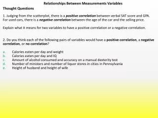
Correlation Analysis • Correlations can be calculated for Categorical variables and Scalar variables • For the former the values range from 0 to 1 and for the latter from –1 to 1 • For Scalar variables, correlations indicate both direction and degree • Positive Correlation (for scalar var):Tendency for a high value of one variable to be associated with a high value in thesecond
Correlation Analysis Sample Correlation (r) • Measure is based on a sample • Reflects tendency for points to cluster systematically about a straight line on a scatter diagram - rising from left to right means positive association - falling from left to right means negative association • r lies between -1 < r < + 1 • r = o means absence of linear association
Correlation Coefficient in practice • Issues to consider - Are the data straight or linear - Is the relationship between the variables significant?
Simple Regression • Moving from association between two variables to predicting value of one from the value of the other • Variable to be predicted is Dependent variable (Y) and variable used to make prediction is Independent variable (X) • Output of regression permits us to: 1. Explain why the values of Y vary as they do 2. Predict Y based on the known values of X
Idea behind Simple Regression • Cataloger wants to know if there is relation between time a customer is on file and sales • Define variables: - Independent var X (Length of time) is number of months since first purchase - Dependent var Y is dollar sales within last month • Draw Scatter plot, draw line through the points and calculate slope of the line • Eye-fitted regression line is Y=10 + 1*X
Fitting the Simple Regression line • Goal is to minimize some measure of variation between Actual observations and Fitted observations • This variation is called Residual Residual =Actual - Fit • The measure of variation is called Residual Sum of Squares • Most common fitting rule called Least-Squares minimizes the Residual Sum of Squares • The equation for simple regression is
Simple Regression in Practice • Turn observations into data (variables) • Access if relationship between X and Y is linear • Straighten out the relationship if needed • Perform the regression analysis using any standard computer program • Interpret the findings
Example • Do customers who buy more frequently also buy bigger ticket items? Step 1. Transform into data as follows: - Independent var (X) is number of purchases in last 12 months - Dependent var (Y) is largest dollar item (LDI) amount
Example (cont) Step 2. Draw Scatter plot to check for linearity Step 3. No straightening out needed Step 4. Regression output is Variation of Y: Variance = 792.94 Total sum of squares = 6343.55 Correlation coefficient: r = 0.97254 Intercept: = -18.22 Regression coefficient: = 10 with p= .001 Regression equation is
Example (cont) Step 5. (i) Large positive value of r indicates strong positive relation between X and Y. (ii) This supports our hypothesis that large sales are associated with frequent purchases (iii) The r squared statistic maybe most important in regression output. Also called Coefficient of Determination. 0 < r < + 1 (iv) Here r squared is .946 (v) Thus 94.6% of variation in Y is explained by X (vi) p value is about significance of
Simple Correlation Co-efficient • Some formulae