Download
1 / 35
350 likes | 387 Views
Learn about scatterplots, association, and correlation between variables, and how to interpret and analyze data using these concepts. Understand the difference between explanatory and response variables and how they can be categorized as categorical or quantitative. Explore examples and scenarios to gain a deeper understanding of these statistical concepts.

E N D
Explanatory and Response Variables The explanatory variable attempts to “explain” the response variable. You would use the explanatory variable to predict the value of the response variable. In a scatterplot, the explanatory variable is always graphed on the horizontal axis.
1.) Identify the explanatory and response variables, and state whether they are categorical or quantitative. a. Researchers measure the heights of children at age 6 and again at age 16. b. A political scientist selects a large sample of registered voters, both male and female, and asks each voter whether they voted for the Democratic or Republican candidate in the last congressional election. c. Breast cancer patients received one of two treatments: (1) removal of the breast or (2) removal of the tumor and lymph nodes only followed by radiation. The patients were followed to see how long they lived following surgery.
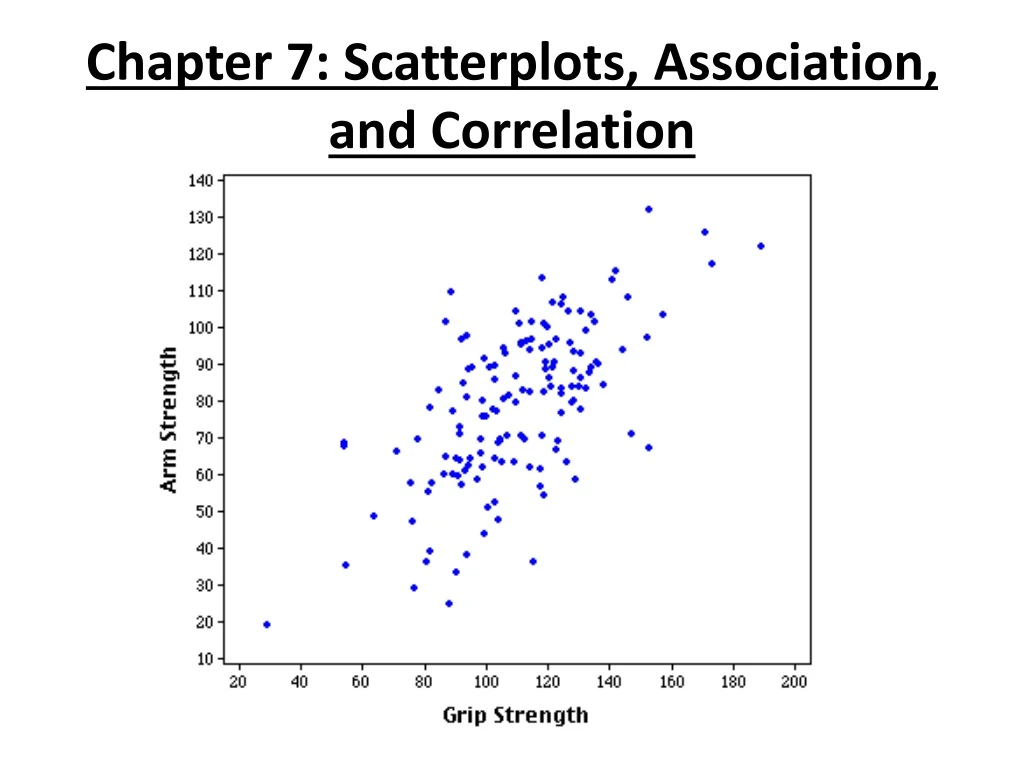
Association in Scatterplots A scatterplot is used to graph the relationship between two quantitative variables for the same individuals. Each individual is represented on the graph by a point . Two variables have a positive association when the both increase or decrease together. Two variables have a negative association when an increase in one variable indicated a decrease in the other. Two variables have no association when the change in one variable cannot be determined from the change in the other.
negative positive none
Slightly Curved Linear Sharply Curved
Moderately Strong Strong: Little to no Scatter Moderately Strong
Clusters (subgroups) Outliers
2. Describe what the scatterplot might look like for each of the following. (a) drug dosage and degree of pain relief (b) calories consumed and weight loss (c) hours of sleep and score on a test (d) shoe size and grade point average (e) time for a mile run and age (f) age of a car and cost of repairs
3. Archaeopteryx is an extinct beast having feathers like a bird but teeth and a long bony tail like a reptile. Only six fossil specimens are known. Because these specimens differ greatly in size, some scientists think they are different species rather than individuals from the same species. If the specimens belong to the same species and differ in size because some are younger than others, there should be a positive linear relationship between the lengths of a pair of bones from all individuals. An outlier would suggest different species. Here are data on the lengths in centimeters of the femur and the humerus for the specimens that preserve both bones: Make a scatterplot. Do you think all five specimens come from the same species?
4. The presence of harmful insects in farm fields is detected by putting up boards covered with a sticky material and then examining the insects trapped on the board. Which colors attract insects best? Experimenters placed six boards of each of four colors in a field of oats and measured the number of cereal leaf beetles trapped. • Create a display of the counts of insects trapped against • board color (space the four colors equally on the • horizontal axis). • Based on the data, what do you conclude about the attractiveness of these colors to the beetles? • What type of association exists between board color and insect count? Explain.
Correlation: Correlation measures the strength and direction of the linear relationship between two quantitative variables. **It is possible to have a strong association but a weak correlation.** Ex. What do you think?
Another name for correlation is the r-value. When there is a positive association between variables, the r-value is positive . When there is a negative association between variables, the r-value is negative . When there is no association between variables, the r-value is about 0 .
The r-value is between -1 and 1 . An r-value of 1 indicates a perfect positive linear relationship; an r-value of -1 indicates a perfect negative linear relationship. An r-value is a standardized value and therefore has no units attached to it. Converting the units of measurement of the data values has no effect on the correlation. The correlation of x with y is the same as the correlation of y with x .
The r-value is greatly affected by outliers . A single outlier can change the strength and direction of the correlation. EX: Find the correlation between the length of the femur and humerus form specimens of Archaeopteryx (refer to #3). Then add in a another set where the femur measure 5 cm and the humerus measured 105 cm. What is the correlation now?
5. If women always married men who were two years older than themselves, what would be the correlation between the ages of husband and wife? • 6. If the lengths of bones were measured in inches instead of centimeters, how would the correlation change? • 7. Each of the following statements contains a blunder. In each case, explain what is wrong. • “There is a high correlation between the sex of American workers and their income.” • “We found a high correlation (r = 1.09) between students’ ratings of faculty teaching and ratings made by other faculty members.” • “The correlation between planting rate and yield of corn was r = 0.23 bushels.”
Correlation Conditions • Remember! Correlationmeasures the strength of the linear association between two quantitative variables. • Before you use correlation, you must check several conditions: • Quantitative Variables Condition • Straight Enough Condition • Outlier Condition
Correlation Conditions (cont.) • Quantitative Variables Condition: • Correlation applies only to quantitative variables. • Don’t apply correlation to categorical data masquerading as quantitative. • Check that you know the variables’ units and what they measure.
Correlation Conditions (cont.) • Straight Enough Condition: • Correlation measures the strength only of the linear association, and will be misleading if the relationship is not linear. • Thus we only calculate and use the correlation coefficient for linear data.
Correlation Conditions (cont.) • Outlier Condition: • Outliers can distort the correlation dramatically. • An outlier can make an otherwise small correlation look big or hide a large correlation. • It can even give an otherwise positive association a negative correlation coefficient (and vice versa). • When you see an outlier, it’s often a good idea to report the correlations with and without the point.
Correlation Properties • The sign of a correlation coefficient gives the direction of the association. • Correlation is always between –1 and +1. • Correlation can be exactly equal to –1 or +1, but these values are unusual in real data because they mean that all the data points fall exactly on a single straight line. • A correlation near zero corresponds to a weak linear association.
Correlation Properties (cont.) • Correlation treats x and y symmetrically: • The correlation of x with y is the same as the correlation of y with x. • Correlation has no units. • Correlation is not affected by changes in the center or scale of either variable. • Correlation depends only on the z-scores, and they are unaffected by changes in center or scale.
Correlation Properties (cont.) • Correlation measures the strength of the linear association between the two variables. • Variables can have a strong association but still have a small correlation if the association isn’t linear. • Correlation is sensitive to outliers. A single outlying value can make a small correlation large or make a large one small.
Review Question! • Which statistics have we studied so far this year that are resistant? • Which statistics are not resistant?
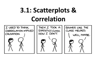
Correlation ≠ Causation • Whenever we have a strong correlation, it is tempting to explain it by imagining that the predictor variable has caused the response to help. • Scatterplots and correlation coefficients never prove causation. • A hidden variable that stands behind a relationship and determines it by simultaneously affecting the other two variables is called a lurking variable.
What Can Go Wrong? • Don’t say “correlation” when you mean “association.” • More often than not, people say correlation when they mean association. • The word “correlation” should be reserved for measuring the strength and direction of the linear relationship between two quantitative variables.
What Can Go Wrong? • Don’t correlate categorical variables. • Be sure to check the Quantitative Variables Condition. • Don’t confuse “correlation” with “causation.” • Scatterplots and correlations never demonstrate causation. • These statistical tools can only demonstrate an association between variables.
What Can Go Wrong? (cont.) • Be sure the association is linear. • There may be a strong association between two variables that have a nonlinear association.
What Can Go Wrong? (cont.) • Don’t assume the relationship is linear just because the correlation coefficient is high. • Here the correlation is 0.979, but the relationship is actually bent.
What Can Go Wrong? (cont.) • Beware of outliers. • Even a single outlier can dominate the correlation value. • Make sure to check the Outlier Condition. • We will discuss outliers in Chapter 8.
What have we learned? • We examine scatterplots for direction, form, strength, and unusual features. • Although not every relationship is linear, when the scatterplot is straight enough, the correlation coefficient is a useful numerical summary. • The sign of the correlation tells us the direction of the association. • The magnitude of the correlation tells us the strength of a linear association. • Correlation has no units, so shifting or scaling the data, standardizing, or swapping the variables has no effect on the numerical value.
What have we learned? (cont.) • Doing Statistics right means that we have to Think about whether our choice of methods is appropriate. • Before finding or talking about a correlation, check the Straight Enough Condition. • Watch out for outliers! • Don’t assume that a high correlation or strong association is evidence of a cause-and-effect relationship—beware of lurking variables!
8. Let’s play Guess the Correlation! http://www.istics.net/Correlations/
AP Tips • Just like the rest of the graphs in this course, scales and labels are required for full credit. • You don’t have to start either axes at zero, but once you start scaling an axes, it should keep the same scale for its entire length. • Describing a scatterplot should be done in context and include the form, strength and association. • “There is a strong, positive, and linear relationship between age and height.”
AP Tips, cont. • We usually refer to r as simply correlation. But the AP test usually refers to r as the correlation coefficient. Don’t get confused by the additional word coefficient. It’s just r.