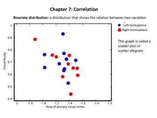
Chapter 7: Correlation

Left hemisphere Right hemisphere Chapter 7: Correlation Bivariate distribution: a distribution that shows the relation between two variables 1 0.9 This graph is called a scatter plot or scatter diagram 0.8 Visual Acuity 0.7 0.6 0.5 0.4 -2 -1.9 -1.8 -1.7 -1.6 -1.5 -1.4 -1.3 Area of primary visual cortex

How do we quantify the strength of the relationship between the two variables in a bivariate distribution?

25 20 Eating Difficulties 15 10 5 5 10 15 20 25 30 35 Stress Example from the book: Two measures made for each subject – stress level and eating difficulties

The most common way to quantify the relation between the two variables in a bivariate distribution is the Pearson correlation coefficient, labeled r. ris always between -1 and 1. The z-score formula is the most intuitive formula: Example: use the z-score formula to calculate r: raw scores z scores zxzyzxzy X Y mx = sx = my = sy = 6.68

How does each data point contribute to the correlation value? mx zxzyzxzy x y r = 0.68 25 20 Eating Difficulties 15 my 10 5 5 10 15 20 25 30 35 30 Stress Points in the upper right or lower left quadrants add to the correlation value Points in the upper left or lower right subtract to the correlation value.

Fun fact about the Pearson correlation statistic Since the z-scores do not change when you add or multiply the raw scores, the Pearson correlation doesn’t change either. multiplying y by 2 and adding 100

r = 0.68 30 25 20 Eating Difficulties 15 r = 0.68 30 10 20 Eating Difficulties 5 10 0 0 5 10 15 20 25 30 0 20 40 Stress Stress Similarly, the correlation stays the same no matter how you stretch your axes: r = 0.68 25 20 As a rule, you should plot your axes with an equal scale. Eating Difficulties 15 10 5 10 20 30 Stress

75 70 65 60 55 50 55 60 65 70 75 80 Guess that correlation! n = 90, r = 0.34 Student's height (in) Average of parent's height (in)

Guess that correlation! n = 21, r = 0.34 78 76 74 Male student's height (in) 72 70 68 66 58 60 62 64 66 68 70 72 Father‘s height (in)

n = 70, r = 0.68 75 70 65 Female student's height (in) 60 55 50 50 55 60 65 70 75 80 85 Mother's height (in)

4 3.5 3 2.5 2.5 3 3.5 4 Guess that correlation! n = 90, r = 0.19 UW GPA High School GPA

11 10 9 8 7 6 5 0 5 10 15 20 25 Guess that correlation! n = 91, r = -0.12 Sleep (hours/night) Caffeine (cups/day)

30 25 20 15 10 5 0 0 5 10 15 20 25 Guess that correlation! n = 91, r = 0.01 Drinks (per week) Caffeine (cups/day)

2000 1800 1600 1400 1200 1000 800 600 400 200 0 0 2 4 6 8 Guess that correlation! n = 91, r = 0.10 Drinks (per week) Facebook friends

5 4.5 4 3.5 3 2.5 2 1.5 1 0.5 0 30 40 50 60 70 80 90 Guess that correlation! n = 91, r = -0.19 Video game playing (hours/week) Favorite outdoor temperature (F)

Guess that correlation! r = -0.56 140 130 120 110 y 100 90 80 70 0 20 40 60 80 100 x

Guess that correlation! r = 0.94 150 145 140 135 130 y 125 120 115 110 105 10 20 30 40 50 60 x

Guess that correlation! r = 0.08 160 150 140 130 y 120 110 100 10 20 30 40 50 60 70 80 90 x

Guess that correlation! r = -1.00 155 150 145 y 140 135 -20 -15 -10 -5 0 5 x

Guess that correlation! r = -0.08 140 130 120 110 y 100 90 80 -40 -30 -20 -10 0 10 20 30 40 x

240 220 200 180 160 140 120 100 80 -50 0 50 100 Guess that correlation! r = 0.49 y x

70 60 50 40 30 20 10 0 -20 -10 0 10 20 30 40 50 60 70 Guess that correlation! r = -0.92 y x

220 210 200 190 180 170 160 150 140 130 -40 -20 0 20 40 60 Guess that correlation! r = -0.77 y x

4 3.5 3 2.5 2 1.5 1 0.5 0 -2 -1 0 1 2 r is a measure of the linear relation between two variables r = 0.01 y x

1 0.5 0 -0.5 -1 -1.5 -1 -0.5 0 0.5 1 1.5 Guess that correlation! r = 0.00 y x

1 0.8 0.6 0.4 0.2 0 -0.2 -0.4 -0.6 -0.8 -1 -1 -0.5 0 0.5 1 Guess that correlation! r = 0.91 y x

Z-Score formula for calculating r (intuitive, but not very practical) Substituting the formula for z: Deviation-Score formula for calculating r: (somewhat intuitive, somewhat more practical) Computational formula for calculating r: (less intuitive, more practical)

Computational formula for calculating r: (less intuitive, more practical) A little algebra shows that: Computational raw score formula for calculating r: (least intuitive, most practical)

Using the Computational raw-score formula:

A second measure of correlation, called the Spearman Rank-Order Coefficient is appropriate for ordinal scores. It is calculated by: Where D is the difference between each pair of ranks. Most often used when: At least one variable is an ordinal scale One of the distributions is very skewed or has outliers

Example: Is there a correlation between your preference for Otter Pops® flavors and mine? Fact: (According to Wikipedia anyway) In 1995, National Pax had planned to replace the "Sir Isaac Lime" flavor with "Scarlett O'Cherry," until a group of Orange County, California fourth-graders created a petition in opposition and picketed the company's headquarters in early 1996. The crusade also included an e-mail campaign, in which a Stanford professor reportedly accused the company of "Otter-cide." After meeting with the children, company executives relented and retained the Sir Isaac Lime flavor.[1]

Example: Suppose two wine experts were asked to rank-order their preference for eight wines. How can we measure the similarity of their rankings?

Pearson correlation is much more sensitive to outlying values than the Spearman coefficient. From: http://en.wikipedia.org/wiki/Spearman%27s_rank_correlation_coefficient

n = 91 Pearson's r = -0.12 Spearman's r = 0.02 s 11 11 10 10 9 9 Sleep (hours/night) 8 8 7 7 6 6 5 5 0 5 10 15 20 0 5 10 15 20 Caffeine (cups/day) Pearson correlation is much more sensitive to outlying values than the Spearman coefficient. n = 89 Pearson's r = 0.06 Spearman's r = 0.07 s Sleep (hours/night) Caffeine (cups/day)

Pearson r: 0.92 Spearman r : 1.00 s 1 0.5 Y 0 -0.5 -0.5 0 0.5 X Only the rank order matters for the Spearman coefficient

Chapter 7: Correlation