Algorithms Problem Solving
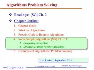
Algorithms Problem Solving. Readings: [SG] Ch. 2 Chapter Outline: Chapter Goals What are Algorithms Pseudo-Code to Express Algorithms Some Simple Algorithms [SG] Ch. 2.3 Computing Array-Sum Structure of Basic Iterative Algorithm Examples of Algorithmic Problem Solving.

Algorithms Problem Solving
E N D
Presentation Transcript
Algorithms Problem Solving • Readings: [SG] Ch. 2 • Chapter Outline: • Chapter Goals • What are Algorithms • Pseudo-Code to Express Algorithms • Some Simple Algorithms [SG] Ch. 2.3 • Computing Array-Sum • Structure of Basic Iterative Algorithm • Examples of Algorithmic Problem Solving Last Revised: September 2013.
Simple iterative algorithm: Array-Sum(A,n) • Input: List of numbers: A1, A2, A3, …., An • Output: To compute the sum of the numbers Note: Store numbers in array A[1], A[2], … , A[n] Array-Sum(A, n); (* Find the sum of A1, A2,…,An. *) begin Sum_SF 0; k 1; while (k <= n) do Sum_SFSum_SF+ A[k]; kk + 1; endwhile Sum Sum_SF; Print“Sum is”, Sum; return Sum; end; Sum_SF representsthe Sum-So-Far
Exercising Algorithm Array-Sum(A,n): A[1] A[2] A[3] A[4] A[5] A[6] n=6 2 5 10 3 12 24 Input: k Sum-SF Sum ? 0 ? 1 2 ? 2 7 ? 3 17 ? 4 20 ? 5 32 ? 6 56 ? 6 56 56 Processing: Output: Sum is 56
Name of Algorithm Parameters: A and n Some comments for human understanding Defining Abstraction Algorithm Array-Sum(A, n); (* Find the sum of A1, A2,…,An. *) begin Sum_SF 0; k 1; while (k <= n) do Sum_SFSum_SF + A[k]; kk + 1; endwhile Sum Sum_SF; return Sum end; Value returned: Sum
Defining a High-level Primitive • Then Array-Sum becomes a high- level primitivedefined as Array-Sum (A, n) Array-Sum A Sum Inputs to Array-Sum: any array A, variablen Outputs from Array-Sum: variableSum n • Definition: Array-Sum (A, n)The high-level primitive Array-Sum takes in as input any array A, a variable n, and it computes and returns the sum of A[1..n], namely, (A[1] + A[2] + . . . + A[n]). These are the inputs to Array-Sum; namely Array A, variable n.
Using a High-level Primitive • First, we define Array-Sum (A, n)The high-level primitive Array-Sum takes in as input any array A, a variable n, and it computes and returns the sum of A[1..n], namely, (A[1] + A[2] + . . . + A[n]). • To use the high-level primitive (or just primitive, in short) we just issue a call to that high-level primitive • Example 1: Array-Sum (A, 6)call the primitive Array-Sum to compute the sum of A[1 .. 6], and returns the sum as its value • Example 2: Top Array-Sum (B, 8)“compute the sum of B[1 .. 8], and store that in variable Top • Example 3: DD Array-Sum (C, m)“compute the sum of C[1 .. m], and store that in variable DD
Using a High-level Primitive • First, we define Array-Sum (A, n)The high-level primitive Array-Sum takes in as input any array A, a variable n, and it computes and returns the sum of A[1..n], namely, (A[1] + A[2] + . . . + A[n]). • To use the high-level primitive (or just primitive, in short) we just issue a call to that high-level primitive • GOOD POINT #1: Can call it many times, no need to rewrite the code • GOOD POINT #2: Can call it to calculate sum of different arrays (sub-arrays) of diff. lengths
Summary: Higher-level Primitive • The algorithm for Array-Sum (A, n) becomes a high- level primitive Array-Sum A Sum n • Can be re-used by (shared with) other people • Machines with this high-level primitive has more capability
Recap: Defining & using high-level primitive • When we do a common task often, we define a high-level primitive to perform the task; • Give it a good name (that suggest what it does); specify what inputs it require, and what outputs it will produce; • Then we can call the high-level primitives each time we need to perform that common task; • In this way, we have extended the capability of “the computer”
Algorithms (Introduction) • Readings: [SG] Ch. 2 • Chapter Outline: • Chapter Goals • What are Algorithms • Pseudo-Code to Express Algorithms • Some Simple Algorithms • Examples of Algorithmic Problem Solving [Ch. 2.3] • Searching Example, • Finding Maximum/Largest • Modular Program Design • Pattern Matching
Structure of “basic iterative algorithm” Algorithm Array-Sum(A, n); (* Find the sum of A1, A2,…,An. *) begin Sum_SF 0; k 1; while (k <= n) do Sum_SFSum_SF + A[k]; kk + 1; endwhile Sum Sum_SF; return Sum end; Initialization block Iteration block; the key step where most of the work is done Post-Processing block Recall Recurring Principle: The Power of Iterations Structure ofBasic iterative algorithm
Re-use of “basic iterative algorithm” • Once an algorithm is developed, • Give it a name (an abstraction): Array-Sum(A, n) • It can be re-used in solving more complex problems • It can be modified to solve other similar problems • Modify algorithm for Array-Sum(A,n) to… • Calculate the average and sum-of-squares • Search for a number; find the max, min • Develop a algorithm library • A collection of useful algorithms • An important tool-kit for algorithm development
Algorithmic Problem Solving • Examples of algorithmic problem solving • Sequential search: find a particular value in an unordered collection • Find maximum: find the largest value in a collection of data • Pattern matching: determine if and where a particular pattern occurs in a piece of text
An Lookup Problem An unordered telephone Directory with 10,000 names and phone numbers TASK: Look up the telephone number of a particular person. ALGORITHMIC TASK: Give an algorithm toLook up the telephone number of a particular person.
Task 1: Looking, Looking, Looking… • Given: An unordered telephone directory • Task • Look up the telephone number of a particular person from an unordered list of telephone subscribers • Algorithm outline • Start with the first entry and check its name, then repeat the process for all entries
Task 1: Looking, Looking, Looking… • Sequential search algorithm • Re-usesthe basic iterative algorithm Array-Sum(A, n) • Refers to a value in the list using an indexi (or pointer/subscript) • Uses the variable Found to exit the iteration as soon as a match is found • Handles special cases • like a name not found in the collection • Question: What to change in Initialization, Iteration, Post-Processing?
Task 1: Sequential Search Algorithm Initialization block Iteration block; the key step where most of the work is done Post-Processing block Figure 2.9: The Sequential Search Algorithm
Algorithm Sequential Search (revised) • Preconditions: The variables NAME, m, and the arrays N[1..m] and T[1..m] have been read into memory. Algorithm Seq-Search (N, T,m, NAME); begin i 1; Found No; while (Found = No) and (i <=m) do if (NAME = N[i]) thenPrintT[i]; Found Yes; elseii + 1; endif endwhile if (Found=No) then Print NAME “is not found” endif return Found, i; end; Initialization block Iteration block; the key step where most of the work is done Post-Processing block
Defining another High-level Primitive • Then Seq-Search becomes a high- level primitivedefined as Seq-Search (N, T, m, Name) Outputs (more than one) Inputs Seq-Search N, T Found m Loc Definition: Seq-Search (N, T, m, Name)The high-level primitive Seq-Search takes in two input arrays N (storing name), and T(storing telephone #s), m the size of the arrays, and Name, the name to search; and return the variables Found and Loc. NAME These are the inputs to Array-Sum; namely Array A, variable n.
Using a High-level Primitive Definition: Seq-Search (N, T, m, Name)The high-level primitive Seq-Search takes in two input arrays N (storing name), and T(storing telephone #s), m the size of the arrays, and Name, the name to search; and return the variable Found and Loc. • To use the high-level primitive (or just primitive, in short) we just issue a call to that high-level primitive • Example 1: Seq-Search (N, T, 100, “John Olson”)call the Seq-Search to find “John Olson” in array N[1 .. 100]. • Example 2: Top Array-Sum (B, 8)“compute the sum of B[1 .. 8], and store that in variable Top
Task 2: Big, Bigger, Biggest Task: • Find the largest value from a list of values Find-Max A Max n Loc • Definition: Find-Max (A, n)The high-level primitive Find-Max takes in as input any array A, a variable n, and it finds and returns variable Max, the maximum element in the array A[1..n], found in location Loc.
Task 2: Big, Bigger, Biggest Task: • Find the largest value from a list of values • Algorithm outline • Keep track of the largest value seen so far • Initialize: Set Largest-So-Far to be the first in the list • Iteration: Compare each value to the Largest-So-Far, and keep the larger as the new largest • Use location to remember where the largest is. • Initialize: … (Do it yourself) • Iteration: …. (Do it yourself)
Task 2: Finding the Largest Initialization block Iteration block; the key step where most of the work is done Figure 2.10: Algorithm to Find the Largest Value in a List Post-Processing block
Algorithm Find-Max • Preconditions: The variable n and the arrays A have been read into memory. Find-Max(A,n); (* find max of A[1..n] *) begin Max-SF A[1]; Location 1; i 2; (* why 2, not 1? *) while (i <= n) do if (A[i] > Max-SF) then Max-SF A[i]; Location i; endif ii + 1 endwhile Max Max-SF; returnMax, Location end; Initialization block Iteration block; the key step where most of the work is done Post-Processing block
Modular Program Design • Software are complex • HUGE (millions of lines of code) eg: Linux, Outlook • COMPLEX; eg: Flight simulator • Idea: Decomposition • Complex tasks can be divided and • Each part solved separately and combined later. • Modular Program Design • Divide big programs into smaller modules • The smaller parts are • called modules, subroutines, or procedures • Design, implement, and test separately • Modularity, Abstraction, Division of Labour • Simplifies process of writing alg/programs
1 2 3 4 5 6 7 8 9 S C A T A T C A T A A T A P Output of Pattern Matching Algorithm: 1 2 3 There is a match at position 2 There is a match at position 7 Task 3: Pattern Matching • Algorithm search for a pattern in a source text Given: A source text S[1..n] and a pattern P[1..m] Question: Find all occurrence of pattern P in text S?
k 1 2 3 4 5 6 7 8 9 S C A T A T C A T A A T A P 1 2 3 Example of Pattern Matching • Align pattern P with text S starting at pos k = 1; • Check for match (between S[1..3] and P[1..3]) • Result – no match
k 1 2 3 4 5 6 7 8 9 S C A T A T C A T A A T A P 1 2 3 Example of Pattern Matching • Align pattern P with text S starting at pos k =2; • Check for match (between S[2..4] and P[1..3]) • Result – match! • Output: There is a match at position 2
k 1 2 3 4 5 6 7 8 9 S C A T A T C A T A A T A P 1 2 3 Example of Pattern Matching • Align pattern P with text S starting at pos k =3; • Check for match (between S[3..5] and P[1..3]) • Result – No match.
k 1 2 3 4 5 6 7 8 9 S C A T A T C A T A A T A P 1 2 3 Example of Pattern Matching • Align pattern P with text S starting at pos k =4; • Check for match (between S[4..6] and P[1..3]) • Result – No match.
k 1 2 3 4 5 6 7 8 9 S C A T A T C A T A A T A P 1 2 3 Example of Pattern Matching • Align pattern P with text S starting at pos k =5; • Check for match (between S[5..7] and P[1..3]) • Result – No match.
Align S[k..(k+m–1)]with P[1..m] k 1 2 3 4 5 6 7 8 9 S C A T A T C A T A A T A P 1 2 3 Example of Pattern Matching • Align pattern P with text S starting at pos k =6; • Check for match (between S[6..8] and P[1..3]) • Result – No match.
k 1 2 3 4 5 6 7 8 9 S C A T A T C A T A A T A P 1 2 3 Example of Pattern Matching Note:k = 7 is the lastposition to test; After that S is “too short”. In general, it is k = n–m+1 • Align pattern P with text S starting at pos k =7; • Check for match (between S[7..9] and P[1..3]) • Result – match! • Output: There is a match at position 7
Yes if S[k..k+m–1] = P[1..m] No otherwise Match(S, k, P, m) = Pattern Matching: Decomposition Task: Find all occurrences of the pattern P in text S; • Algorithm Design: Top Down Decomposition • Modify from basic iterative algorithm (index k) • At each iterative step (for each k) • Align pattern P with S at position k and • Test for match between P[1..m] and S[k .. k+m –1] • Define an abstraction (“high level operation”)
Use the “high level operation” Match(S,k,P,m) which can be refined later. Pattern Matching: Pat-Match • Preconditions: The variables n, m, and the arrays S and P have been read into memory. Pat-Match(S,n,P,m); (* Finds all occurrences of P in S *) begin k 1; while (k <= n-m+1) do if Match(S,k,P,m) = Yes thenPrint “Match at pos ”, k; endif k k+1; endwhile end;
i 1 2 3 4 5 6 7 8 9 S C A T A T C A T A A T A P 1 2 3 Match of S[k..k+m-1] and P[1..m] Align S[k..k+m–1]with P[1..m] (Here, k = 4) Match(S,k,P,m); begin i 1; MisMatch No; while (i <= m) and (MisMatch=No) do if (S[k+i-1] not equal to P[i]) thenMisMatch=Yes elseii + 1 endif endwhile Match not(MisMatch); return Match end;
i 1 2 3 4 5 6 7 8 9 S C A T A T C A T A A T A P 1 2 3 Example: Match of S[4..6] and P[1..3] Align S[k..k+m–1]with P[1..m] (Here, k = 4) • [k = 4] With i= 1,MisMatch = No • Compare S[4] and P[1] (S[k+i-1] and P[i]) • They are equal, so increment i
i 1 2 3 4 5 6 7 8 9 S C A T A T C A T A A T A P 1 2 3 Example: Match of S[4..6] and P[1..3] Align S[k..k+m–1]with P[1..m] (Here, k = 4) • [k = 4] With i= 2,MisMatch = No • Compare S[5] and P[2] (S[k+i-1] and P[i]) • They are equal, so increment i
i 1 2 3 4 5 6 7 8 9 S C A T A T C A T A A T A P 1 2 3 Example: Match of T[4..6] and P[1..3] Align S[k..k+m–1]with P[1..m] (Here, k = 4) • [k = 4] With i= 3,MisMatch = No • Compare S[6] and P[3] (S[k+i-1] and P[i]) • They are not equal, so set MisMatch=Yes
Our Top-Down Design • Our pattern matching alg. consists of two modules • Achieves good division-of-labour • Made use of top-down design and abstraction • Separate “high-level” view from “low-level” details • Make difficult problems more manageable • Allows piece-by-piece development of algorithms • Key concept in computer science Pat-Match(S,n,P,m) “higher-level” view Match(S,k,P,m) “high-level” primitive
Use the “high level primitive operation” Match(S,k,P,m) which can be de/refined later. Pattern Matching: Pat-Match (1st draft) • Preconditions: The variables n, m, and the arrays S and P have been read into memory. Pat-Match(S,n,P,m); (* Finds all occurrences of P in S *) begin k 1; while (k <= n-m+1) do if Match(S,k,P,m) = Yes thenPrint “Match at pos ”, k; endif k k+1; endwhile end;
Pattern Matching Algorithm of [SG] THINK:: How can Mismatch=NO here? This part compute Match(T,k,P,m) Figure 2.12: Final Draft of the Pattern-Matching Algorithm
Pattern Matching Algorithm of [SG] • Pattern-matching algorithm • Contains a loop within a loop • External loop iterates through possible locations of matches to pattern • Internal loop iterates through corresponding characters of pattern and string to evaluate match
Summary • Specify algorithms using pseudo-code • Unambiguous, readable, analyzable • Algorithm specified by three types of operations • Sequential, conditional, and repetitive operations • Seen several examples of algorithm design • Designing algorithm is not so hard • Re-use, Modify/Adapt, Abstract your algorithms • Algorithm design is also a creative process • Top-down design helps manage complexity • Process-oriented thinking helps too
Summary • Importance of “doing it” • Test out each algorithm to find out “what is really happening” • Run some of the animations in the lecture notes • If you are new to algorithms • read the textbook • try out the algorithms • do the exercises … The End …