Genetic Algorithms in Problem Solving
Genetic Algorithms in Problem Solving. 1998 년 7 월 16 일 조 동 연. EVOLVING COMPUTER PROGRAMS (1). Evolving Lisp Programs Kepler’s Third Law: P 2 = cA 3. PROGRAM ORBITAL_PERIORD C # Mars # A = 1.52 P = SQRT(A * A * A) PRINT P END ORBITAL_PERIORD. (defun orbital_period () ; Mars ;

Genetic Algorithms in Problem Solving
E N D
Presentation Transcript
Genetic Algorithms in Problem Solving 1998년 7월 16일 조 동 연
EVOLVING COMPUTER PROGRAMS (1) • Evolving Lisp Programs • Kepler’s Third Law: P2 = cA3 PROGRAM ORBITAL_PERIORD C # Mars # A = 1.52 P = SQRT(A * A * A) PRINT P END ORBITAL_PERIORD (defun orbital_period () ; Mars ; (setf A 1.52) (sqrt (* A (* A A))))
EVOLVING COMPUTER PROGRAMS (2) • Koza’s algorithm - Genetic Programming (GP) 1. Choose a set of possible functions and terminals for the program. F = {+, - *, /, }, T = {A} 2. Generate an initial population of random trees (programs) using the set of possible functions and terminals. 3. Calculate the fitness of each program in the population by running it on a set of “fitness cases” (a set of input for which the correct output is known). 4. Apply selection, crossover, and mutation to the population to form a new population. 5. Steps 3 and 4 are repeated for some number of generations.
EVOLVING COMPUTER PROGRAMS (4) • Block-Stacking Problem • T = {CS, TB, NN} • F = {MS(x), MT(x), DU(exp1, exp2), NOT(exp1), EQ(exp1, exp2) } • (EQ (DU (MT CS) (NOT CS)) (DU (MS NN) (NOT NN)))
EVOLVING COMPUTER PROGRAMS (5) • Evolving Cellular Automata (CA) • Example (N=11, radius = 1) • space-time diagram Rule table: neighborhood: 000 001 010 011 100 101 110 111 output bit : 0 0 0 1 0 1 1 1 Lattice: t = 0 1 0 1 0 0 1 1 1 0 1 0 t = 1 0 1 0 0 0 1 1 1 1 0 1
EVOLVING COMPUTER PROGRAMS (6) • Density-classification task (N=149, r =3)
DATA ANALYSIS AND PREDICTION (1) • Predicting Dynamical Systems • individual • C = {($20 Price of Xerox Stock on day 1) ^ ($25 Price of Xerox Stock on day 2 $27) ^ ($22 Price of Xerox Stock on day 3 $25)} • crossover, mutation
DATA ANALYSIS AND PREDICTION (3) • Predicting Protein Structure
EVOLVING NEURAL NETWORKS (2) • Evolving Weights in a Fixed Network
EVOLVING NEURAL NETWORKS (4) • Evolving Network Architectures • Direct Encoding
EVOLVING NEURAL NETWORKS (5) • Grammatical Encoding