Download
1 / 58
580 likes | 606 Views
Dive into the realm of wave optics with topics like Huygens’ Principle, polarization, interference, diffraction, and Fourier optics. Unravel the complexities of optical systems and their significance in various applications.

E N D
EDAYATHANKUDY G S PILLAY ARTS AND SCIENCE COLLAGEWave Optics W.CHRISTPHER IMMANWELL
Spherical Wave, Image Formation, and Huygens’ Principle Wavefront: a surface over which the phase of a wave is constant Huygens’ Principle
Reflection and Transmittance of Polarized Lights Fresnel equations: Note: p-polarization: E-field plane of incidence s-polarization: E-field plane of incidence
Antireflection Film Antireflection Coatings on Solar Cells
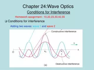
Interference Young’s Experiment Interference — superposition of two light wave result in bright and dark fringes Conditions for Interference: • same polarization • same frequency • constant phase relationship (coherence)
Conditions for Interference Bright fringes: = 0, 2, 4,…(in phase) Dark fringes: = , 3, 5, …(out of phase) If 1 = 2 =
Fabry-Perot Interferometer (Cont’) GaAs’s natural cleavage plane is (1,1,0)-plane. Si’s and Ge’s natural cleavage plane are (1,1,1)-plane.
Recording process Reconstructionprocess Holography/Hologram
Sagnac Effect and Ring Interferometer N: Fringe number
Interferences of Coherent/Incoherent Waves • Coherence: All component electromagnetic waves are in phase or in the same phase difference. • Interference ofcoherent waves: Waves of different frequencies interfere to form a pulse if they are coherent. • Interference ofincoherent waves: Spectrally incoherent light interferes to form continuous light with a randomly varying phase and amplitude.
Resolving Power of Imaging Systems Rayleigh criterion
Minimum resolvable angular: D: diameter of open aperture : wavelength of light source Note: if < min, images cannot be resolved Minimum resolvable separation: where =h/d1 For objective lens, numerical aperture NA=sin1 Resolution Limit • Rayleigh criterion two object point can be resolved by the lens of an optical system
Resolution of Human Eye Resolving power of human eye 0.3 mrad Resolution limit of human eye 0.075mm
Optical Fourier Transform Fourier Plane Input Plane FTL f f a(x,y) A(u,v)
Fourier Optics and Its applications Optical Computing
Coherence Function Mutually coherent: point sources u1(t1, x1, y1, z1) and u2(t1, x2, y2, z2) maintain a fixed phase relation Mutual coherence function: Normalized mutual coherence function: (complex degree of coherence or degree of correlation) where 11() and 22() are the self-coherence functions of u1(t) and u2(t)
Demonstration of Coherence Visibility of fringe: extended source interference pattern If I1 = I2= I (best condition), = 12() i.e., visibility of the fringe is a measure of the degree of coherence
Spatial Coherence extended source Intensity distribution of the resultant fringe of two points on the extended source: extended source
Temporal Coherence Visibility of the fringe is a measure of the degree of temporal coherence 11() at same point Coherence length of the light source