Download
1 / 56
560 likes | 677 Views
Long Run Projections for Climate Change Scenarios. Warwick J McKibbin ANU, Lowy Institute and Brookings David Pearce Centre for International Economics Alison Stegman Australian National University. Prepared for the International Symposium on Forecasting conference, Sydney July 7, 2004.

E N D
Long Run Projections for Climate Change Scenarios Warwick J McKibbin ANU, Lowy Institute and Brookings David Pearce Centre for International Economics Alison Stegman Australian National University Prepared for the International Symposium on Forecasting conference, Sydney July 7, 2004
Structure of Presentation • Overview • Some Theoretical Issues • Sources of growth • Convergence (of what?) Across countries • Theory • Empirical evidence • Measurement Issues • Purchasing Power Parity (PPP) versus Market Exchange Rates (MER) • The G-Cubed Approach of making projections • Overview • Sensitivity to productivity assumptions • Sensitivity to PPP versus MER convergence assumptions • The Intergovernmental Panel on Climate Change (IPCC) Special Report on Emissions Scenarios (SRES) Approach • Conclusion
A Comment on the climate debate: • Some argue that climate change doesn’t exist, that the science is wrong, that nothing should be done • Some argue that climate change is so important that there is no cost too high to tackle the problem • Both approaches are likely to be wrong • Good public policy must recognize the risks as well as the costs to society of the responses.
What is Climate policy about ? • We know that carbon concentrations in the atmosphere have risen 30% since the industrial revolution. • We know the science of the greenhouse effect. Everything else is uncertain: • Uncertainty about link between carbon dioxide emissions and the timing and magnitude of climate change • Uncertainty about costs and benefits of climate change • Uncertainty about costs and benefits of abatement • Uncertainty about the policy responses
Why emission projections matter • Critical input into climate change debate • Policies have been and are being conditioned on the baseline and initial conditions • Emission projections feed into climate models to make temperature projections • Temperature projections feed into impact models to assess – environmental/ecological/economic/health impacts over the next century
What do we Know? • Not enough to precisely condition policies on our projections • Problem is that the overwhelming importance of uncertainty is not addressed in most proposed policies • Particularly not in the Kyoto Protocol • McKibbin/Wilcoxen Blueprint does address the issue of optimal climate policy under uncertainty • See McKibbin W. and P. Wilcoxen (2002) ‘The Role of Economics in Climate Change Policy”, Journal of Economic Perspectives, vol 16, no 2, pp107-130.
What do we Know? Oil price shocks of the 1970s generated important information for estimating the impacts of energy prices on economic behavior • Supply (substitution, technical change) • Demand (conservation, substitution)
Interpretation • Economic Modelers use this as evidence that relative prices matter – (and estimate the effects) • Energy modelers tend to use the data post 1975 to calculate “Autonomous Energy Efficiency Improvements” • In projecting the future, it matters a great deal which approach is followed.
Theoretical Issues in Forecasting Growth • Sources of output growth • Increases in the supply capital, labor, energy, materials • Increase in the quality of these inputs • Improvements in the way the inputs are used (technical change) • Improvements in the way inputs are allocated across the economy • Improvements in the way inputs are allocated across the world
Theoretical Issues in Forecasting Global Growth • Convergence • What converges? • Incomes per capita • GDP per capita • Aggregate level or rate of technical progress • Sectoral level or rates of technical progress • The empirical literature examines conditional versus unconditional convergence of income per capita and to a lesser extent output per worker (productivity) • Little empirical evidence of unconditional convergence across large numbers of countries
Theoretical Issues related to PPP (purchasing power parity) • International comparisons of incomes per capita should be undertaken in a common unit. • Market exchange rates are not a good way to convert incomes. • PPPs have been developed to enable conversions of volumes of goods into common units. • PPP is a measurement concept not the theoretical proposition that exchange rates will adjust to equalize relative prices across countries • Various ways to calculate PPP and they each give different results but all are clustered together relative to market exchange rates
Theoretical Issues • PPP versus market exchange rates • Castles and Henderson argue that if the rate of growth of developing countries are measured based on the initial differences in income per capita then it is critical to measure this gap using PPP • Many studies use market exchange rates and so growth is likely to be overestimated. • Empirical illustration of this point later.
The G-Cubed Approach McKibbin & Wilcoxen
The G-Cubed Model • Countries • United States • Japan • Australia • New Zealand • Canada • Rest of OECD • Brazil • Rest of Latin America • China • India • Eastern Europe and Former Soviet Union • Oil Exporting Developing Countries • Other non Oil Exporting Developing Countries
The G-Cubed Model • Sectors • (1) Electric Utilities • (2) Gas Utilities • (3) Petroleum Refining • (4) Coal Mining • (5) Crude Oil and Gas Extraction • (6) Other Mining • (7) Agriculture, Fishing and Hunting • (8) Forestry and Wood Products • (9) Durable Manufacturing • (10) Non Durable Manufacturing • (11) Transportation • (12) Services • (Y) capital good producing sector
Features of the G-Cubed Model • Dynamic • Intertemporal • General Equilibrium • Multi-Country • Multi-sectoral • Econometric • Macroeconomic
G-Cubed Approach to Projections • Bagnoli, P. McKibbin W. and P. Wilcoxen (1996) “Future Projections and Structural Change” in N, Nakicenovic, W. Nordhaus, R. Richels and F. Toth (ed) Climate Change: Integrating Economics and Policy, CP 96-1 , International Institute for Applied Systems Analysis (Austria), pp181-206.
G-Cubed Approach of Generating Future Projections • Make assumptions about labor augmenting technical change (LATC) for each sector in the US • Calculate economy wide gaps between LATC within each sector relative to the US sector such that the TFP gap across sectors is approximately equal to the PPP GDP per worker gap • Assume that the gap in LATC between each country and the US closes by 2% per year (i.e. the Barro rate)
Process of Generating Future Projections • Assume that labor supply grows at the rate of the mid range UN population projections from 2002 to 2050 and then gradually converges across countries to zero population growth in the long run. • Other exogenous inputs include tax rates per country per sector, tariff rates per country per sector, monetary and fiscal regimes
Process of Generating Future Projections • Given initial capital stocks in each sector, the overall output growth rate of an economy depends; • the growth on LATC (exogenous), • labor force (exogenous in the long run); • the accumulation of capital (endogenous) • the use of materials input by type (endogenous) • the use of energy inputs by type (endogenous)
Key Points • The projection of carbon emissions will depend on the growth of the demand for carbon intensive inputs (oil, natural gas, coal). • There is no reason for a fixed relationship between growth in the economy and growth in carbon emissions • The outcomes depend on the trend inputs and the structural change in the economy induced on the supply side and demand side of all economies.
Key Points • In Bagnoli, McKibbin and Wilcoxen (1996) we showed that if all sectors were assumed to follow the same LATC growth versus the case where all sectors followed the historical experience of LATC growth, scaled to give the same overall GDP growth for the US economy, then carbon emissions in the case of equal sectoral growth would be double the case of differential sectoral growth after 30 years.
An Illustration • Suppose there is increase GDP growth because of sectoral productivity growth that differs across sectors. What happens to emissions growth? • Things to examine: • The impact of US growth on US Emissions • The impact of US growth on other countries emissions • The impact of foreign growth on US emissions
An Illustration • The following slides examine the change in carbon emissions in 2020 and 2050 relative to BAU as a result of productivity growth in each sector, sector by sector
The G-Cubed Model • Sectors • (1) Electric Utilities • (2) Gas Utilities • (3) Petroleum Refining • (4) Coal Mining • (5) Crude Oil and Gas Extraction • (6) Other Mining • (7) Agriculture, Fishing and Hunting • (8) Forestry and Wood Products • (9) Durable Manufacturing • (10) Non Durable Manufacturing • (11) Transportation • (12) Services • (Y) capital good producing sector
Key Points • For global emissions it matters which sector in which country experiences productivity growth • Models that assume constant ratios or linear trends between GDP and emissions are likely to be problematic if the actual growth process involves structural change
PPP versus Market Exchange Rates • G-Cubed uses a PPP concept for GDP to benchmark the initial productivity gap between sectors in each country relative to the US • The rate of economic growth and emissions outcomes are determined simultaneously • Suppose we use market exchange rates to benchmark initial gaps between countries – what difference does this make to emission projections?
An Example • The ratio of the productivity of China to the US is 0.2 based on PPP • The ratio of the productivity of LDCs to the US is 0.4 based on PPP • Suppose we assume • China has an initial gap of 0.1 (from MER) • LDCs have a gap of 0.13 (from MER)
Implications • PPP versus market exchange rates makes a big difference to the projections of economic growth and the projections of future carbon emissions • The errors affect both developing and developed countries • Does this matter for temperature? • Manne and Richels argue that temperature is based on the stock of cumulative emissions and flows take time to have any impact • BUT these magnitudes are to large for the IPCC to dismiss the way they have to date.
The SRES Approach • Intergovernmental Panel on Climate Change (IPCC) • Special Report on Emissions Scenarios (SRES) • SRES report contains scenarios to provide “input for evaluating climatic and environmental consequences of future greenhouse emissions and for assessing alternative mitigation adaptation strategies”
The SRES Approach • Focus on 4 regions although projections actually undertaken at greater detail: • OECD90 • Ref (reform countries of Eastern Europe and former Soviet Union) • ASIA (developing countries in Asia) • ALM (developing countries in Africa, Latin Am and Middle East)
The SRES Approach • Develop a range of “qualitative storylines” that focus on the main drivers of greenhouse gas emissions • Demographic change, social and economic development, and rate and direction of technological change • No assessment of likelihood of these scenarios.
What underlies these projections? • Growth assumptions • AEEI assumptions • Population assumptions
The Response of the SRES Authors to Critiques • Convergence is not assumed in most scenarios (not clear what is assumed) • Doesn’t matter whether convergence is defined in PPP or MER one can always convert between the two (problem is that there is no empirical relationship) • Even where convergence is assumed, it is not clear that assuming high growth in developing countries would cause emissions to be overestimated because with higher income there would be more investment in technology and more emissions reductions • How plausible is this argument?
IPAT Identity (Erlich and Holdren) Impact = Population Affluence Technology Emissions = Population GDP/capita Emissions/GDP E = PGDPPC I (Emissions Intensity) In growth rates: e = p + gdppc + i
Problem with conventional use of this relation • GDP per capita and Emissions per unit of GDP are both endogenous • Suppose we assume a CES production function of energy and non energy inputs • Energy is a CES function of Carbon emitting and non-emitting technologies
This equation Shows • Change in emission intensity depends on • Change in relative prices of energy and non-energy inputs; • Changes in relative prices of emitting and non emitting energy sources; • and the ability to substitute between these • It is possible to GDP to rise and emissions to fall • Problem for the Energy models in the SRES is that they generally assume no substitution so GDP and emissions should are more likely to move together than in G-Cubed • It comes back to exogenous changes in AEEI offsetting higher growth