Download
1 / 34
390 likes | 758 Views
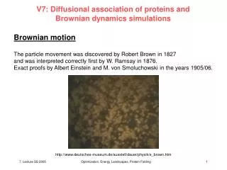
V7: Diffusional association of proteins and Brownian dynamics simulations. Brownian motion The particle movement was discovered by Robert Brown in 1827 and was interpreted correctly first by W. Ramsay in 1876. Exact proofs by Albert Einstein and M. von Smoluchowski in the years 1905/06.

E N D
V7: Diffusional association of proteins and Brownian dynamics simulations Brownian motion The particle movement was discovered by Robert Brown in 1827 and was interpreted correctly first by W. Ramsay in 1876. Exact proofs by Albert Einstein and M. von Smoluchowski in the years 1905/06. http://www.deutsches-museum.de/ausstell/dauer/physik/e_brown.htm Optimization, Energy Landscapes, Protein Folding
t = 24 s t = 0 s 0.5 mm Diffusion of 2 mm particles in water and DNA solution Diffusion of 0.5 mm particles in water Diffusion - Brownian dynamics http://www.deas.harvard.edu/projects/weitzlab/research/micrheo.html Optimization, Energy Landscapes, Protein Folding
: stochastic force Hydrodynamics:x is the friction constant h: viscosity a: radius of the particle m: mass of the particle Statistical calculations: Einstein relation Langevin equation Theory of stochastic processes: -> colloidal suspensions (particles in a liquid) more collisions in the front than in the back => force in opposite direction and proportional to velocity: Optimization, Energy Landscapes, Protein Folding
Fick’s 1st law Flux of particles in 1D: in 3D: Fick’s 1st law + conservation of particles -> Diffusion equation in 1D: in 3D: (Fick’s 2nd law) … considering the friction force Smoluchowski equation Smoluchowski equation Optimization, Energy Landscapes, Protein Folding
U(r) r a b Kramer’s Theory Transition state theory assumptions: - thermodynamic equilibrium in the entire system - transition from reactant state which crosses the transition state will end in the product state Kramers (1940): escape rate for strong (over-damped) friction (large x) Optimization, Energy Landscapes, Protein Folding
steady state: Diffusion equation: (without friction) after integrating: particle flux: number of collisions per second at r = a: association rate: Protein-protein association Protein-protein association is crucial in cellular processes like signal transduction, immune response, etc. Diffusive association of particles to a sphere ~ 109 M-1s-1 Optimization, Energy Landscapes, Protein Folding
Protein-protein association II a more realistic scenario … typical association rates ~ 103 - 109 M-1s-1 barnase / barstar Optimization, Energy Landscapes, Protein Folding
Short range interactions: • van der Waals forces • hydrophobic interactions • formation of atomic contacts • structure of water molecules • Long range interactions: • electrostatic forces • desolvation forces • hydrodynamic interactions • Entropic effects: • (restriction of the degrees of freedom) • translational entropy • rotational entropy • side chain entropy Forces between the proteins Optimization, Energy Landscapes, Protein Folding
BD MD The association pathway Steps involved in protein-protein association: • random diffusion • electrostatic steering • formation of encounter complex • dissociation or formation of final complex Association pathway depends on: • forces between the proteins • solvent properties like temperature, ionic strength Optimization, Energy Landscapes, Protein Folding
Diffusional motion of a particle Translational / rotational diffusion coefficients D / DR Translational displacement during each time step: with and Rotational displacement during each time step : with and Brownian dynamics simulations Ermak-McCammon-Algorithm: Optimization, Energy Landscapes, Protein Folding
SDA Simulation of Diffusional Association of proteins Gabdoulline and Wade, (1998) Methods, 14, 329-341 Optimization, Energy Landscapes, Protein Folding
Example trajectory barstar barnase Optimization, Energy Landscapes, Protein Folding
Example system: barnase / barstar barnase • barnase: a ribonuclease that acts extracellularlybarstar: its intracellular inhibitordiameters of both ~ 30 Å • provides well-characterized model system of electrostatically steered diffusional encounter between proteins • interaction between barnase and barstar is among the strongest known interactions between proteins • very fast association rate: 108 – 109 M-1s-1 at 50 mM ionic strength • simulated rates are in good agreement with experimental results barstar - 7 kT/e + 7 kT/e Optimization, Energy Landscapes, Protein Folding
d1-2 orientation: qn q 30° 30° 60° 60° 90° 90° Computation of the occupancy landscape d1-2 position: Optimization, Energy Landscapes, Protein Folding
Results: Occupancy landscape bound complex: d1-2 = 23.8 Å Optimization, Energy Landscapes, Protein Folding
center-center distance d1-2: minimum distance between contact pairs cdmin: distance between geometric centers of contact surfaces cdcenter: average distance between contact pairs cdavg: global view detailed view Choice of the distance axis Optimization, Energy Landscapes, Protein Folding
Results: Occupancy landscape II bound complex: cdavg = 3.56 Å Optimization, Energy Landscapes, Protein Folding
Entropy from occupancy maps Occupancy maps can be interpreted as probability distributions for the computation of an entropy landscape Proteins can only explore the surrounding region entropy for each grid point is calculated from the probability distribution within accessible volumes V and Y Take V as sphere with radiusDr, Y as sphere with radiusDw around protein position and orientation Average displacement within BD time step ofDt ~ 1 ps: In the simulations:Dr = 3 Å,Dw= 3° Optimization, Energy Landscapes, Protein Folding
Basic entropy formula applied for all states within V and Y: Dr Entropy from occupancy maps II Entropy of a system with N states: probability for each state if all states are equally probable, Pn = 1/N: Entropy in protein-protein encounter: Optimization, Energy Landscapes, Protein Folding
Free energy landscape bound complex: d1-2 = 23.8 Å Optimization, Energy Landscapes, Protein Folding
Results: Occupancy landscape II bound complex: d1-2 = 23.8 Å Optimization, Energy Landscapes, Protein Folding
Energy profiles DEel -TDS DEds DG encounter state Optimization, Energy Landscapes, Protein Folding
Encounter complex free energy: DG = -4.053 kcal/mol Optimization, Energy Landscapes, Protein Folding
Encounter complex II free energy: DG = -4.0 kcal/mol volume of encounter region: Venc = 14.4 Å3 lifetime: Dt = 2.1 ps Optimization, Energy Landscapes, Protein Folding
Encounter complex III free energy: DG = -3.5 kcal/mol volume of encounter region: Venc = 1492 Å3 lifetime: Dt = 11.5 ps Optimization, Energy Landscapes, Protein Folding
Encounter complex IV free energy: DG = -3.0 kcal/mol volume of encounter region: Venc = 5338 Å3 lifetime: Dt = 20.1 ps Optimization, Energy Landscapes, Protein Folding
Encounter complex V free energy: DG = -2.8 kcal/mol volume of encounter region: Venc = 8377 Å3 lifetime: Dt = 18.5 ps Optimization, Energy Landscapes, Protein Folding
Encounter regions: comparison regions for energetically favourable regions for each protein from BD simulations: DG ≤ -3 kcal/mol from a Boltzmann factor analysis Gabdoulline & Wade: JMB (2001) 306:1139 Optimization, Energy Landscapes, Protein Folding
Encounter regions: comparison II regions for energetically favourable regions for each protein from BD simulations: DG ≤ -2.5 kcal/mol from a Boltzmann factor analysis Gabdoulline & Wade: JMB (2001) 306:1139 Optimization, Energy Landscapes, Protein Folding
Association pathways paths of highest occupancy vs. paths of lowest free energy Optimization, Energy Landscapes, Protein Folding
Coupling of translation and orientation Optimization, Energy Landscapes, Protein Folding
-TDS DEel ---- WT ---- E60A ---- K27A ---- R59A ---- R83Q ---- R87A 83 27 87 59 60 DG DEds Mutant effects Energy Profiles: Optimization, Energy Landscapes, Protein Folding
83 27 87 59 60 Mutant effects II Encounter Regions: DG ¡ÂDGmin + 0.5 kcal/mol WT E60A K27A R59A R83Q R87A DG ---- WT ---- E60A ---- K27A ---- R59A ---- R83Q ---- R87A Optimization, Energy Landscapes, Protein Folding
Summary • Brownian motion: • Particles in solutions move according to a random force • average displacement: • Association: • association of spherical particles -> ‘diffusion limit’, • protein association is steered along the free energy funnel • Interactions: • long-range association can be modeled by BD simulation, • short-range association by MD simulation • BD simulations allow • the calculation of association rates • analysis of association paths • identification of the encounter complex Optimization, Energy Landscapes, Protein Folding