Download
1 / 30
300 likes | 428 Views
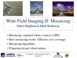
Wide Field Imaging II: Mosaicing Debra Shepherd & Mark Holdaway. Mosaicing: required when a source is BIG. How mosaicing works: Effective ( uv ) coverage Mosaicing algorithms Preparing mosaic observations. Mosaicing Overlapping Fields. Surveys for point sources

E N D
Wide Field Imaging II: MosaicingDebra Shepherd & Mark Holdaway Mosaicing: required when a source is BIG. How mosaicing works: Effective (uv) coverage Mosaicing algorithms Preparing mosaic observations D. Shepherd, Synthesis Summer School, June 2002
Mosaicing Overlapping Fields Surveys for point sources Serpens 3 mm continuum: Image extended emission G192.16 CO(J=1-0) outflow: D. Shepherd, Synthesis Summer School, June 2002
Mosaicing Adding Zero Spacing Flux G75.78 star forming region in CO(J=1-0) BIMA + 12m = Combined Interferometric Mosaic 12m BIMA 12m + BIMA D. Shepherd, Synthesis Summer School, June 2002
How big is “BIG”? • Bigger than the Primary Beam:/D Full Width Half Max • Bigger than what the shortest baseline can measure: Largest angular scale in arcsec, LAS = 91,000/Bshort • VLA short baselines can recover: • 80% flux on 1/5/D Gaussian; 50% on 1/3/D Gaussian • CLEAN can do well on a 1/2/D Gaussian • MEM can still do well on a high SNR 1/2/D Gaussian • Lack of short baselines often become a problem before source structure is larger than the primary beam: Mosaicing is almost always about Total Power! D. Shepherd, Synthesis Summer School, June 2002
LAS • LASis a function of wavelength: • VLA at 21 cm (L band): 15’ • VLA at 3.6 cm (X band): 3’ • VLA at 0.7 cm (Q band): 40” • OVRO at 2.7 mm (115 GHz): 20” • ALMA at 1 mm (230 GHz): 13” • ALMA at 0.4 mm (690 GHz): 4” • Mosaicing becomes more critical at short wavelengths. D. Shepherd, Synthesis Summer School, June 2002
An Example • Assume a model brightness distribution: I(x) • Simulated visibilities are given by: • V(u) = mm (A(x – xp) I(x)) e -2pi(u .x) dx • Estimate of brightness distribution at a single pointing is: • I recon(x) / A(x – xp) • Need more pointings! D. Shepherd, Synthesis Summer School, June 2002
An Example: Simulated Data I(x) * BG(x) Image smoothed with 6” Gaussian (VLA D config. resolution at 15 GHz) I(x) Raw model brightness distribution D. Shepherd, Synthesis Summer School, June 2002
An Example: Simulated Data A(x – xp) Primary beam used for simulations A(x – xp) I(x) * BG(x) Model multiplied by primary beam & smoothed with 6” Gaussian. Best we can hope to reconstruct from single pointing. D. Shepherd, Synthesis Summer School, June 2002
An Example: Reconstructed Simulated Data I recon(x) / A(x – xp) Primary beam-corrected image. Blanked for beam response < 10% peak. Need to Mosaic! I recon(x) Visibilities constructed with thermal Gaussian noise. Image Fourier transformed & deconvolved with MEM D. Shepherd, Synthesis Summer School, June 2002
Effective uv coverage – How Mosaicing Works • Single dish: scan across source, Fourier transform image to get information out to dish diameter, D: • Ekers & Rots (1979): One visibility = linear combination of visibilities obtained from patches on each antenna: • But, can’t solve for N unknowns (Fourier information on many points between b-D & b+D) with only one piece of data (a single visibility measurement). Need more data! Density of uv points (u,v) Single dish Single baseline D. Shepherd, Synthesis Summer School, June 2002
How Mosaicing Works • Ekers & Rots obtained the information between spacings b-D & b+D by scanning the interferometer over the source and Fourier transforming the single baseline visibility with respect to the pointing position. So, changing the pointing position on the sky is equivalent to introducing a phase gradient in the uv plane. This effectively smooths out the sampling distribution in the uv plane: Snapshot coverage Effective mosaic coverage v(kl) u(kl) u(kl) D. Shepherd, Synthesis Summer School, June 2002
Example: Simulated Mosaic • Try 9 pointings on simulated data. We could deconvolve each field separately and knit together in a linear mosaic using: • Imos(x) = ________________ • But, Cornwell (1985) showed that one can get much better results by using all the data together to make a single image through joint deconvolution. • In practice, if spacings close to the dish diameter can be measured (b ~ D), then the “effective” Fourier plane coverage in a mosaic allows us to recover spacings up to about ½ a dish diameter. Still need Total Power. Sp A(x – xp) Ip(x) Sp A2(x – xp) D. Shepherd, Synthesis Summer School, June 2002
An Example: Reconstructed Simulated Data Nine VLA pointings deconvolved via a non-linear mosaic algorithm (AIPS VTESS). No total power included. Same mosaic with total power added. D. Shepherd, Synthesis Summer School, June 2002
Interferometers & Single Dishes Array VLA ATCA OVRO BIMA PdBI Number Ants 27 6 6 10 6 Diameter (m) 25 22 10.4 6.1 15 Bshort (m) 35 24 15 7 24 Single Dish GBT or VLBA Parks IRAM or GBT 12m, IRAM or GBT IRAM Diameter (m) 100 25 64 30 100 12, 30 100 30 D. Shepherd, Synthesis Summer School, June 2002
Mosaics in Practice W75 N molecular outflow, CO(J=1-0). (Stark, Shepherd, & Testi 2002) 17 OVRO pointings deconvolved via a non-linear mosaic algorithm (MIRIAD mosmem). No total power included. D. Shepherd, Synthesis Summer School, June 2002
Mosaics in Practice Crab Nebula at 8.4 GHz. (Cornwell, Holdaway, & Uson 1993). VLA + Total power from a VLBA antenna D. Shepherd, Synthesis Summer School, June 2002
Non-Linear Joint Deconvolution • Find dirty image consistent with ALL data. Optimize global c2: • c2 = S________________ • The gradient of c2 w.r.t. the model image tells us how to change the model so c2 is reduced: • Like a mosaic of the residual images; use to steer optimization engine like non-linear deconvolver MEM. AIPS:vtess & utess. ˆ |V(ui,xp) – V(ui,xp)|2 i,p s 2 (ui,xp) Point spread fctn Global model image Dirty image Primary beam c2 (x) = -2Sp A(x – xp) {Ip,(x) – Bp(x) *[A(x – xp) I(x)]} D Residual image for pointing p D. Shepherd, Synthesis Summer School, June 2002
Joint Deconvolution (Sault et al.(1996) • Dirty images from each pointing are linearly mosaiced. An image-plane weighting function is constructed that results in constant thermal noise across the image (source structure at the edge of the sensitivity pattern is not imaged at full flux). • Dirty beams stored in a cube. c2 (x) residual image is formed and used in MEM and CLEAN-based deconvolution algorithms. • Final images restored using model intensity & residuals. MIRIAD: invert; mosmem or mossdi; restore. D. Shepherd, Synthesis Summer School, June 2002
Linear Mosaic of Dirty Images with Subsequent Joint Deconvolution • Limited dynamic range (few hundred to one) due to position dependent PSF. AIPS: ltess • This can be fixed by splitting the deconvolution into major and minor cycles. Then subtracting the believable deconvolved emission from the data and re-mosaicing the residual visibilities. AIPS++: imager D. Shepherd, Synthesis Summer School, June 2002
Linear Mosaic + Joint Deconvolution with Major/Minor Cycles • Dirty images from each pointing are linearly mosaiced. AIPS++: imager • Approximate point spread function is created common to all pointings. Assures uniform PSF across mosaic. • Image deconvolved until approx. PSF differs from true PSF for each pointing by specified amount. Model is subtracted from the observed data (in visibility or image plane) to get residual image. Iterations continue until peak residual is less than cutoff level. • AIPS++ deconvolution algorithms are input function to imager: mem, clean, msclean. mscleansimultaneously cleans N different component sizes to recover compact & extended structure. D. Shepherd, Synthesis Summer School, June 2002
Challenges: - Low declination source, - bright point sources, - faint extended emission. Relic radio galaxy 1401-33. (Goss et al. 2002) ATCA L band mosaic, 11 fields, deconvolved with AIPS++, multi-scale clean. No total power included. D. Shepherd, Synthesis Summer School, June 2002
Adding in total power Total power obtained from a single dish telescope can be: • Added in uv plane (MIRIAD: invert). Single dish image must be Fourier transformed to create simulated uv coverage: Example: HI in the SMC. • “Feathered” together after images are made (AIPS++: image.feather, MIRIAD: immerge) IF there is sufficient uv overlap between interferometer and single dish data (VLA+GBT, OVRO/BIMA+IRAM, ATCA+Parkes): Examples: MIRIAD: Galactic center CS(2-1), AIPS++:Orion. Caution: if the single dish pointing accuracy is poor, then the combined image can be significantly degraded. The only single dish that can produce images of similar quality to what an interferometer can produce is the GBT. D. Shepherd, Synthesis Summer School, June 2002
G75.78 star forming region in CO(J=1-0) Kitt Peak 12m image convolved with BIMA primary beam, converted to uv data with sampling density similar to BIMA uv coverage, scaled & combined with BIMA data, inverted with a taper, joint deconvolution (MIRIAD). Kitt Peak 12m BIMA 12m + BIMA Shepherd, Churchwell, & Wilner (1997) D. Shepherd, Synthesis Summer School, June 2002
Linear Image “Feathering” - immerge If there is significant overlap in uv-coverage: images can be “feathered” together in the Fourier plane. Merged data Interferometer ATCA mosaic Parkes Single dish MIRIAD immerge tapers low spatial frequencies of mosaic interferometer data to increase resolution while preserving flux. Can taper interferometer data to compensate. D. Shepherd, Synthesis Summer School, June 2002
MIRIAD mosaic of the SMC ATCA observations of HI in the SMC. Dirty mosaic, interferometer only. Deconvolved mosaic, interferometer only. Stanimirovic et al. (1999). D. Shepherd, Synthesis Summer School, June 2002
MIRIAD mosaic of the SMC Total power image from Parkes. Interferometer plus single dish feathered together (immerge). Stanimirovic et al. (1999). D. Shepherd, Synthesis Summer School, June 2002
CS(2-1) Near the Galactic Center OVRO mosaic, 4 fields. Deconvolved with MEM. OVRO+IRAM 30m mosaic using MIRIAD: immerge feather algorithm. Lang et al. 2001. D. Shepherd, Synthesis Summer School, June 2002
Ionized Gas (8.4 GHz) in the Orion Nebula GBT On-the-fly map of the large field, (AIPS++). 90” resolution. VLA mosaic of central region, 9 fields. Deconvolved with MEM in AIPS++. 8.4” resolution. GBT+VLA mosaic using AIPS++ image.feather. Shepherd, Maddalena, McMullin, 2002. Dissimilar resolution is a problem in all total power combo techniques currently available – plans to develop multi-scale SD+interferometer deconvolution in AIPS++! D. Shepherd, Synthesis Summer School, June 2002
Good Mosaic Practice • Point in the right place on the sky. • Nyquist sample the sky: pointing separation l/2D • Observe extra pointings in a guard band around source. • If extended structure exists, get total power information. Have good uv overlap between single dish and interferometer (big single dish w/ good pointing/low sidelobes & short baselines). • Observe short integrations of all pointing centers, repeat mosaic cycle to get good uv coverage and calibration until desired integration time is achieved. • For VLA: Either specify each pointing center as a different source or use //OF (offset) cards to minimize set up time. D. Shepherd, Synthesis Summer School, June 2002
W50 Supernova Remnant (Dubner et al. 1998) D. Shepherd, Synthesis Summer School, June 2002