Download
1 / 164
1.74k likes | 2k Views
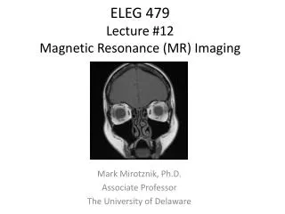
ELEG 479 Lecture #12 Magnetic Resonance (MR) Imaging. Mark Mirotznik, Ph.D. Associate Professor The University of Delaware. Physics of Magnetic Resonance Summary. Protons and electrons have a property called spin that results in them looking like tiny magnets. . N. N. S. =. No Net

E N D
ELEG 479Lecture #12Magnetic Resonance (MR) Imaging Mark Mirotznik, Ph.D. Associate Professor The University of Delaware
Physics of Magnetic ResonanceSummary • Protons and electrons have a property called spin that results in them looking like tiny magnets. N N S = No Net Magnetization S • In the absence of an external magnetic field all the magnetic dipole are oriented randomly so we get zero net magnetic field when we add them all up. Random Orientation
Physics of Magnetic ResonanceSummary • When we add a large external magnetic field we can get the protons to line up in 1 of 2 orientations (spin up or spin down) with a few more per million in one of the orientations than the other. This produces a net magnetization along the axis of the applied magnetic field. • When we add a large external magnetic field we cause a torque on the already spinning proton that causes it to precess like a top around the applied magnetic field. The frequency is precesses , called its Larmor frequency., is determined from Larmor’s equation.
Physics of Magnetic ResonanceSummary from Last Lecture The net magnetization vector is the sum of all of these little magnetic moments added together. This is what we measure. z z z y y x x y z z x Net Magnetization Vector y y x x
Physics of Magnetic ResonanceSummary from Last Lecture • However since all the spinning protons are precessing out of phase with each other this results in zero net magnetization in the transverse plane. = 0 This is bad news since is where are signal comes from! Somehow we need to get these guys spinning together!
Physics of Magnetic ResonanceSummary from Last Lecture To get them to all spin together we add a RF field whose frequency is the same as the Larmor resonant frequency of the proton and is oriented in the xy or transverse plane. B1 RF Excitation time B1
Physics of Magnetic ResonanceSummary from Last Lecture B1 a a B1Dt z Time of Application of RF Pulse Tip Angle Amplitude of RF Pulse y x
Physics of Magnetic ResonanceSummary from Last Lecture a = envelope of the RF signal z In general y x
Physics of Magnetic ResonanceSummary from Last Lecture • To get the signal out we place a coil near the sample. A time-varying transverse magnetic field will produce a voltage on the coil that can be digitized and stored for processing. recall and
Physics of Magnetic ResonanceRelaxation • After the RF field is removed over time the spin system will return back to it’s equilibrium state due to several relaxation processes.
Physics of Magnetic ResonanceRelaxation • After the RF field is removed over time the spin system will return back to it’s equilibrium state due to several relaxation processes. These are: • Spin-Spin relaxation (also called the T2 relaxation): Due to random processes in which neighboring proton spins effect each other spin system will lose coherence and Mxy will decay. This is an irreversible process. • Spin-Lattice relaxation (also called T1relaxation): Due to another random process the Mz will begin to recover back to it’s original equilibrium state. Also irreversible. • T2* relaxation: Due to inhomogenities in the external Bo field Mxy will decay much faster than T2. This is a reversible process.
T2 Decay RF RF
T2*Decay: Dephasing due to field inhomogeneity z' y' = 0 Mxy x' T2*relaxation is dephasingoftransverse magnetization too but it turns out to be reversible
MRI Image • An MRI image is determined by two things • three intrinsic properties of the tissue. These are: T1, T2and Pd. (two relaxation time constants and the density of protons) • the details of the external magnetic fields (Bo, B1 and the gradient magnetics (have not talked about these yet)). How they are configured and how we turn them on and off (pulse sequence) effects what the image looks like. • By varying the pulse sequence we can control which of the intrinsic properties to emphasize in the image.
TR 180 degree RF pulses 0.5TE 0.5TE 0.5TE 0.5TE 90 degree RF pulses TE TE White matter T1=813 ms T2=101 ms
TR 180 degree RF pulses CASE I: TR>>T1 , TE<T2 What do we measure? 90 degree RF pulses TE TE White matter T1=813 ms T2=101 ms
CASE I: TR>>T1 , TE<T2 • Short TE means that the signal has not decayed much due to T2relaxation. • Long TR means that by the next pulse the system is back at equilibrium (Mz due to T1 relaxation has fully recovered) • So what are we measuring? TR 180 degree RF pulses 90 degree RF pulses TE TE White matter T1=813 ms T2=101 ms
CASE I: TR>>T1 , TE<T2 • Short TE means that the signal has not decayed much due to T2relaxation. • Long TR means that by the next pulse the system is back at equilibrium (Mz due to T1 relaxation has fully recovered) • So what are we measuring? • PD Weighted imaging! TR 180 degree RF pulses 90 degree RF pulses TE TE White matter T1=813 ms T2=101 ms
TR 180 degree RF pulses CASE II: TR>>T1 , TE~T2 90 degree RF pulses TE TE White matter T1=813 ms T2=101 ms
CASE II: TR>>T1 , TE~T2 • TE on the order of T2means that the signal is proportional to the T2relaxation constant. • Long TR means that by the next pulse the system is back at equilibrium (Mz due to T1 relaxation has fully recovered) • So what are we measuring? TR 180 degree RF pulses 90 degree RF pulses TE TE White matter T1=813 ms T2=101 ms
CASE II: TR>>T1 , TE~T2 • TE on the order of T2means that the signal is proportional to the T2relaxation constant. • Long TR means that by the next pulse the system is back at equilibrium (Mz due to T1 relaxation has fully recovered) • So what are we measuring? • T2 Weighted imaging! TR 180 degree RF pulses 90 degree RF pulses TE TE White matter T1=813 ms T2=101 ms
TR CASE III: TR~T1 , TE<T2 What do we measure? 180 degree RF pulses 90 degree RF pulses TE
CASE III: TR~T1 , TE<T2 • TE is shorter than T2means that the signal is not heavily weighted on the T2relaxation constant. • TR on the order of T1 means that by the next pulse the system is not back at equilibrium (Mz due to T1 relaxation has not fully recovered) • So what are we measuring? TR 180 degree RF pulses 90 degree RF pulses TE
CASE III: TR~T1 , TE<T2 • TE is shorter than T2means that the signal is not heavily weighted on the T2relaxation constant. • TR on the order of T1 means that by the next pulse the system is not back at equilibrium (Mz due to T1 relaxation has not fully recovered) • So what are we measuring? • T1 Weighted imaging! TR 180 degree RF pulses 90 degree RF pulses TE
Tissue Contrast Summary
Full Bloch equation including relaxation precession, RF excitation longitudinal magnetization transverse magnetization includes Boand B1
Example: Solve for the transverse components of M after a 90 degree pulse.
Example: Solve for the transverse components of M after a 90 degree pulse. After 90 degree pulse the RF field is shut down and only Bo is non-zero
Example: Solve for the transverse components of M after a 90 degree pulse. After 90 degree pulse the RF field is shut down and only Bo is non-zero Initial conditions for 90 degree pulse:
Example: Solve for the transverse components of M after a 90 degree pulse. After 90 degree pulse the RF field is shut down and only Bo is non-zero Solutions
Example: Solve for the transverse components of M after a 90 degree pulse. After 90 degree pulse the RF field is shut down and only Bo is non-zero Solutions
Example: Solve for the transverse components of M after an arbitrary flip angle (a) After an arbitrary RF pulse the RF field is shut down and only Bo is non-zero
Example: Solve for the transverse components of M after an arbitrary flip angle (a) After an arbitrary RF pulse the RF field is shut down and only Bo is non-zero Initial conditions for 90 degree pulse:
Example: Solve for the transverse components of M after an arbitrary flip angle (a) Solutions
Solve full Bloch equation with only B=Bo Solution for transverse components Mx and My Where a is the flip angle after RF excitation