Stereo
Stereo. CSE 455 Ali Farhadi Several slides from Larry Zitnick and Steve Seitz. Why do we perceive depth?. What do humans use as depth cues?. Motion. Convergence


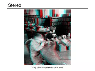
Stereo
E N D
Presentation Transcript
Stereo CSE 455 Ali Farhadi Several slides from Larry Zitnick and Steve Seitz
What do humans use as depth cues? Motion Convergence When watching an object close to us, our eyes point slightly inward. This difference in the direction of the eyes is called convergence. This depth cue is effective only on short distances (less than 10 meters). Binocular Parallax As our eyes see the world from slightly different locations, the images sensed by the eyes are slightly different. This difference in the sensed images is called binocular parallax. Human visual system is very sensitive to these differences, and binocular parallax is the most important depth cue for medium viewing distances. The sense of depth can be achieved using binocular parallax even if all other depth cues are removed. Monocular Movement Parallax If we close one of our eyes, we can perceive depth by moving our head. This happens because human visual system can extract depth information in two similar images sensed after each other, in the same way it can combine two images from different eyes. Focus Accommodation Accommodation is the tension of the muscle that changes the focal length of the lens of eye. Thus it brings into focus objects at different distances. This depth cue is quite weak, and it is effective only at short viewing distances (less than 2 meters) and with other cues. Marko Teittinenhttp://www.hitl.washington.edu/scivw/EVE/III.A.1.c.DepthCues.html
What do humans use as depth cues? Image cues Retinal Image Size When the real size of the object is known, our brain compares the sensed size of the object to this real size, and thus acquires information about the distance of the object. Linear Perspective When looking down a straight level road we see the parallel sides of the road meet in the horizon. This effect is often visible in photos and it is an important depth cue. It is called linear perspective. Texture Gradient The closer we are to an object the more detail we can see of its surface texture. So objects with smooth textures are usually interpreted being farther away. This is especially true if the surface texture spans all the distance from near to far. Overlapping When objects block each other out of our sight, we know that the object that blocks the other one is closer to us. The object whose outline pattern looks more continuous is felt to lie closer. Aerial Haze The mountains in the horizon look always slightly bluish or hazy. The reason for this are small water and dust particles in the air between the eye and the mountains. The farther the mountains, the hazier they look. Shades and Shadows When we know the location of a light source and see objects casting shadows on other objects, we learn that the object shadowing the other is closer to the light source. As most illumination comes downward we tend to resolve ambiguities using this information. The three dimensional looking computer user interfaces are a nice example on this. Also, bright objects seem to be closer to the observer than dark ones. Jonathan Chiu Marko Teittinenhttp://www.hitl.washington.edu/scivw/EVE/III.A.1.c.DepthCues.html
Amount of horizontal movement is … …inversely proportional to the distance from the camera
X z x x’ f f BaselineB C C’ Depth from Stereo X • Goal: recover depth by finding image coordinate x’ that corresponds to x x x'
Depth from disparity X z x x’ f f BaselineB O O’ Disparity is inversely proportional to depth.
Depth from Stereo X • Goal: recover depth by finding image coordinate x’ that corresponds to x • Sub-Problems • Calibration: How do we recover the relation of the cameras (if not already known)? • Correspondence: How do we search for the matching point x’? x x'
Correspondence Problem • We have two images taken from cameras with different intrinsic and extrinsic parameters • How do we match a point in the first image to a point in the second? How can we constrain our search? x ?
Key idea: Epipolar constraint X X X x x’ x’ x’ Potential matches for x have to lie on the corresponding line l’. Potential matches for x’ have to lie on the corresponding line l.
Epipolar geometry: notation X x x’ • Baseline – line connecting the two camera centers • Epipoles • = intersections of baseline with image planes • = projections of the other camera center • Epipolar Plane – plane containing baseline (1D family)
Epipolar geometry: notation X x x’ • Baseline – line connecting the two camera centers • Epipoles • = intersections of baseline with image planes • = projections of the other camera center • Epipolar Plane – plane containing baseline (1D family) • Epipolar Lines - intersections of epipolar plane with image planes (always come in corresponding pairs)
Example: Forward motion What would the epipolar lines look like if the camera moves directly forward?
Example: Motion perpendicular to image plane • Points move along lines radiating from the epipole: “focus of expansion” • Epipole is the principal point
Example: Forward motion e’ e Epipole has same coordinates in both images. Points move along lines radiating from “Focus of expansion”
Epipolar constraint • If we observe a point x in one image, where can the corresponding point x’ be in the other image? X x x’
Epipolar constraint X X X x x’ x’ x’ • Potential matches for x have to lie on the corresponding • epipolar line l’. • Potential matches for x’have to lie on the corresponding • epipolar line l.
Epipolar constraint: Calibrated case • Assume that the intrinsic and extrinsic parameters of the cameras are known • We can multiply the projection matrix of each camera (and the image points) by the inverse of the calibration matrix to get normalized image coordinates • We can also set the global coordinate system to the coordinate system of the first camera. Then the projection matrices of the two cameras can be written as [I | 0] and [R | t] X x x’
Epipolar constraint: Calibrated case X = (x,1)T x x’ = Rx+t t R The vectors Rx, t, and x’ are coplanar
Epipolar constraint: Calibrated case X x x’ Essential Matrix (Longuet-Higgins, 1981) The vectors Rx, t, and x’ are coplanar
Epipolar constraint: Calibrated case • E x is the epipolar line associated with x(l' = E x) • ETx'is the epipolar line associated with x'(l = ETx') • E e= 0 and ETe' = 0 • Eis singular (rank two) • E has five degrees of freedom X x x’
Epipolar constraint: Uncalibrated case • The calibration matrices K and K’ of the two cameras are unknown • We can write the epipolar constraint in terms of unknown normalized coordinates: X x x’
Epipolar constraint: Uncalibrated case X x x’ Fundamental Matrix (Faugeras and Luong, 1992)
Epipolar constraint: Uncalibrated case X x x’ • F xis the epipolar line associated with x(l' = F x) • FTx'is the epipolar line associated with x'(l' = FTx') • F e= 0 and FTe'= 0 • Fis singular (rank two) • F has seven degrees of freedom
Minimize: under the constraint||F||2=1 The eight-point algorithm A Smallest eigenvalue of ATA
The eight-point algorithm • Meaning of errorsum of squared algebraic distances between points x’iand epipolar lines Fxi (or points xi and epipolar lines FTx’i) • Nonlinear approach: minimize sum of squared geometric distances
Problem with eight-point algorithm • Poor numerical conditioning • Can be fixed by rescaling the data
The normalized eight-point algorithm • Center the image data at the origin, and scale it so the mean squared distance between the origin and the data points is 2 pixels • Use the eight-point algorithm to compute F from the normalized points • Enforce the rank-2 constraint (for example, take SVD of F and throw out the smallest singular value) • Transform fundamental matrix back to original units: if T and T’ are the normalizing transformations in the two images, then the fundamental matrix in original coordinates is T’TF T (Hartley, 1995)
Moving on to stereo… Fuse a calibrated binocular stereo pair to produce a depth image image 1 image 2 Dense depth map Many of these slides adapted from Steve Seitz and Lana Lazebnik
Depth from disparity X z x x’ f f BaselineB O O’ Disparity is inversely proportional to depth.
Basic stereo matching algorithm • If necessary, rectify the two stereo images to transform epipolar lines into scanlines • For each pixel x in the first image • Find corresponding epipolarscanline in the right image • Search the scanline and pick the best match x’ • Compute disparity x-x’ and set depth(x) = fB/(x-x’)
Simplest Case: Parallel images Epipolar constraint: R = I t = (T, 0, 0) x x’ t The y-coordinates of corresponding points are the same
Stereo image rectification • Reproject image planes onto a common plane parallel to the line between camera centers • Pixel motion is horizontal after this transformation • Two homographies (3x3 transform), one for each input image reprojection • C. Loop and Z. Zhang. Computing Rectifying Homographies for Stereo Vision. IEEE Conf. Computer Vision and Pattern Recognition, 1999.
Example Unrectified Rectified
Correspondence search • Slide a window along the right scanline and compare contents of that window with the reference window in the left image • Matching cost: SSD or normalized correlation Left Right scanline Matching cost disparity
Correspondence search Left Right scanline SSD
Correspondence search Left Right scanline Norm. corr
Effect of window size W = 3 W = 20 • Smaller window + More detail • More noise • Larger window + Smoother disparity maps • Less detail • Fails near boundaries
Failures of correspondence search Occlusions, repetition Textureless surfaces Non-Lambertian surfaces, specularities
Results with window search Data Window-based matching Ground truth
How can we improve window-based matching? • So far, matches are independent for each point • What constraints or priors can we add?