Stereo
Stereo. Course web page: vision.cis.udel.edu/~cv. April 16, 2003 Lecture 22. Announcements . Read Forsyth & Ponce, Chapter 17-17.2 on tracking for Friday HW4 assigned today is due on Monday, April 28. Outline. Estimating the fundamental matrix F


Stereo
E N D
Presentation Transcript
Stereo Course web page: vision.cis.udel.edu/~cv April 16, 2003 Lecture 22
Announcements • Read Forsyth & Ponce, Chapter 17-17.2 on tracking for Friday • HW4 assigned today is due on Monday, April 28
Outline • Estimating the fundamental matrix F • DLT with manually chosen correspondences • Nonlinear minimization • Texture mapping • Homework 4
Estimating F • Same general approach as DLT method for camera matrix estimation • Need at least 8 point correspondences for linear method to set up homogeneous system Af = 0 (details in reading) • Key steps • Normalization: Transform points so that • Centroids of points in each image are translated to origin • Points are scaled so that RMS distance (number of standard deviations) to origin is p2 • Solve linear system with SVD method (see last lecture or camera calibration lecture) • Enforce rank constraint • Denormalize • Remember to normalize so that F(3, 3) = 1!
Estimating F: Singularity Constraint • Must enforce singularity constraint so that epipolar lines intersect at one point • Replace F with closest F’ minimizing Frobenius norm kF–F’k such that detF’ = 0 • Can do this easily with SVD: • Let F= UDVT, where D = diag(r, s, t) is diagonal matrix • Then F’ = Udiag(r, s, 0)VT
Example: Epipolar Lines with and without rank 2 constraint from Hartley & Zisserman
Estimating F : Degenerate Configurations • DLT method does not yield a solution when: • Points in the two images are related by a homography • Points and camera are on a ruled quadric (e.g., one hyperboloid, two planes / cones / cylinders)
Measuring Geometric Error • E.g., symmetric epipolar distance: Overall point-to-line distances given by
Nonlinear Iterative Refinement of the F Estimate • Idea: Improve F estimate by minimizing geometric error (e.g., symmetric epipolar distance) with iterative method • Enforcing rank-2 property • Shouldn’t wait until minimization is over and project F onto nearest singular F’ as with DLT • To ensure property holds at each step of minimization: • Penalize deviations from detF= 0 with some constraint function • Or, e.g., over-parametrization: Writing F= [t]£Mfor arbitrary 3 x 3 matrix M guarantees that F is singular. So minimize over the 12 parameters of t, M instead of the 7 of F
Matlab: Nonlinear Iterative Refinement of the F Estimate • Unconstrained nonlinear minimization:fminsearch • Specify starting point x0 (could be F directly or 12 parameters of t, M) • Specify error function f that takes parameters x, a, and b (such as sets of corresponding points) and returns scalar • Answer is x = fminsearch(‘f’,x0,[],a,b) • Constrained nonlinear minimization:fmincon • Can also specify nonlinear constraint function (e.g., use det(F) as penalty)
Image Transformations • Geometric: Compute new pixel locations according to transformation T (x, y) !(x’, y’) • Translation trivial • Rotate, scaling • Undistort (e.g., radial distortion from lens) • Photometric: Computing new pixel values • Forward mapping may leave “holes” • Backward mapping T -1 ensures coverage of target • Computing a value when T -1(x’,y’) non-integral: • Nearest neighbor: Value of closest pixel ! Aliasing • Bilinear interpolation (2 x 2 neighborhood) • Bicubic interpolation (4 x 4) courtesy of S. Becker
Vertical blend Horizontal blend Bilinear Interpolation • Idea: Blend four pixel values surrounding source, weighted by nearness
Texture Mapping:NN vs. Bilinear Interpolation Matlab imrotate 45±, imresize 1.5
Homework 4 • Single view metrology • Plane-to-plane distance • Vanishing point, line computation • Cross ratio • Comparing lengths between planes • Affine rectification • Homology computation • Fundamental matrix estimation • DLT • Nonlinear minimization