Stereo
Stereo . Dan Kong. depth. baseline. Stereo vision. Triangulate on two images of the same scene point to recover depth. Camera calibration Finding all correspondence Computing depth or surfaces. Right. left. Outline. Basic stereo equations Constraints and assumption


Stereo
E N D
Presentation Transcript
Stereo Dan Kong
depth baseline Stereo vision Triangulate on two images of the same scenepoint to recover depth. • Camera calibration • Finding all correspondence • Computing depth or surfaces Right left
Outline • Basic stereo equations • Constraints and assumption • Windows-based matching • Cooperative Stereo • Dynamic programming • Graph cut and Belief Propagation • Segmentation-based method
Pinhole Camera Model Image plane Virtual Image
Basic Stereo Derivations disparity
Stereo Constraint • Color constancy • The color of any world points remains constant from image to image • This assumption is true under Lambertian Model • In practice, given photometric camera calibration and typical scenes, color constancy holds well enough for most stereo algorithms.
Stereo Constraint • Epipolar geometry • The epipolar geometry is the fundamental constraint in stereo. • Rectification aligns epipolar lines with scanlines Epipolar plane Epipolar line for p Epipolar line for p’
Stereo Constraint • Uniqueness and Continuity • Proposed by Marr&Poggio. • Each item from each image may be assigned at most one disparity value,” and the “disparity” varies smoothly almost everywhere.
Correspondence Using Window-based matching scanline Right Left SSD error disparity Left Right
Sum of Squared (Pixel) Differences Left Right
ImageNormalization • Even when the cameras are identical models, there can be differences in gain and sensitivity. • The cameras do not see exactly the same surfaces, so their overall light levels can differ. • For these reasons and more, it is a good idea to normalize the pixels in each window:
Images as Vectors Left Right “Unwrap” image to form vector, using raster scan order row 1 row 2 Each window is a vectorin an m2 dimensionalvector space.Normalization makesthem unit length. row 3
Normalized Correlation Normalized Correlation
Results Usingwindow-based Method Left Disparity Map Images courtesy of Point Grey Research Left Right
Stereo Results Left Disparity map
Problems with Window-based matching • Disparity within the window must be constant. • Bias the results towards frontal-parallel surfaces. • Blur across depth discontinuities. • Perform poorly in textureless regions. • Erroneous results in occluded regions
Cooperative Stereo Algorithm • Based on two basic assumption by Marr and Poggio: • Uniqueness: at most a single unique match exists for each pixel. • Continuous: disparity values are generally continuous, i.e., smooth within a local neighborhood.
Disparity Space Image (DSI) • The 3D disparity space has dimensions row r column c and disparity d. Each element (r, c, d) of the disparity space projects to the pixel (r, c) in the left image and to the (r, c + d) in the right image • DSI represents the confidence or likelihood of a particular match.
Illustration of DSI (r, c) slices for different d (c, d) slice for r = 151
Definition Match value assigned to element (r, c, d) at iteration n Initial values computed from SSD or NCC Inhibition area for element (r, c, d) Local support area for element (r, c, d)
Iterative Updating DSI 1 2 3 4
Explicit Detection of Occlusion Identify occlusions by examining the magnitude of the converged values in conjunction with the uniqueness constrain
Summary of Cooperative Stereo • Prepare a 3D array, (r, c, d): (r, c) for each pixel in the reference image and d for the range of disparity. • Set initial match values using a function of image intensities, such as normalized correlation or SSD. • Iteratively update match values using (4) until the match values converge. • For each pixel (r, c), find the element (r, c, d) with the maximum match value. • If the maximum match value is higher than a threshold, output the disparity d, otherwise, declare a occlusion.
MRF Stereo Model • Local Evidence function • Compatibility function :Lx1 vector :LxL matrix
Disparity Optimization • Joint probability of MRF: • The disparity optimization step requires choosing an estimator for • MMSE: estimate of the mean of the marginal distribution of • MAP: the labeling of maximize the above joint probability (1)
Equivalence to Energy Minimization • Taking the negative log of equation 1: • In graph cut, equation 2 is expressed as: • Maximizing the probability in equation 1is equivalent to minimizing energy in equation 3. (2) (3)
Stereo Matching Using Belief Propagation • Belief propagation is an iterative inference algorithm that propagates messages in the Markov network Message node send to Message observed node send to Belief at node We simplify as , and as
Belief Propagation Algorithm Initialize messages as uniform distribution Iterative update messages for I = 1:T Compute belief at each node and output disparity
Stereo As a Pixel-Labeling Problem • Let P be a set of pixels, L be a label set. The goal is find a labeling f which minimize some energy. For stereo, the labels are disparities. • The classic form of energy function is:
Energy Function: • The energy function measures how appropriate a label is for the pixel given the observed data. In stereo, this term corresponds to the match cost or likelihood. • The energy term encodes the prior or smoothness constraint. In stereo, the so called Potts model is used:
Two Energy Minimization Algorithm via Graph Cuts Swap algorithm
Two Energy Minimization Algorithm via Graph Cuts expansion algorithm
Graph Cuts Results Belief Propagation Graph Cuts
Ordering Constraint • If an object a is left on an object b in the left image then object a will also appear to the left of object b in the right image Ordering constraint… …and its failure
… … Stereo Correspondences Left scanline Right scanline Match intensities sequentially between two scanlines
… … Match Match Match Left occlusion Right occlusion Stereo Correspondences Left scanline Right scanline
Left Occluded Pixels Search Over Correspondences Three cases: • Sequential – cost of match • Left occluded – cost of no match • Right occluded – cost of no match Left scanline Right scanline Right occluded Pixels
Left Occluded Pixels Standard 3-move Dynamic Programming for Stereo Dynamic programming yields the optimal path through grid. This is the best set of matches that satisfy the ordering constraint Left scanline Start Right scanline Right occluded Pixels End
Dynamic Programming • Efficient algorithm for solving sequential decision (optimal path) problems. 1 1 1 1 … 2 2 2 2 3 3 3 3 How many paths through this trellis?
Dynamic Programming 1 1 1 States: 2 2 2 3 3 3 Suppose cost can be decomposed into stages:
Dynamic Programming 1 1 1 2 2 2 3 3 3 Principle of Optimality for an n-stage assignment problem
Dynamic Programming 1 1 1 2 2 2 3 3 3
Stereo Matching with Dynamic Programming Pseudo-code describing how to calculate the optimal match
Stereo Matching with Dynamic Programming Pseudo-code describing how to reconstruct the optimal path
Results Local errors may be propagated along a scan-line and no inter scan-line consistency is enforced.