Download
1 / 14
140 likes | 159 Views
Overview of modeling approach, Linux cluster setup, parallel computing and performance, and features of CMAQ model.

E N D
CCOS Seasonal Modeling:The Computing Environment S.Tonse, N.J.Brown & R. Harley Lawrence Berkeley National Laboratory University Of California at Berkeley
Overview • Modeling Approach • Linux Cluster: OS & hardware • Parallel computing & performance • CMAQ flavours and features
Modeling Approach MM5 model provides 3D gridded spatial/temporal wind vectors, temperature fields, cloud cover etc. MM5 code run by ETL group of NOAA (J.Wilczak et al) CMAQ (Community Multiscale Air Quality) Model (US EPA) incorporates meteorology results from MM5 with emissions. Fortran 90. Runs on Linux platforms with Pentiums or Athlons. 3D time-stepping grid simulation includes atmospheric chemistry and advective and diffusive transport. Provides concentration for each 4km x 4km grid cell at every hour.
Photochemical AQM: (CMAQ). Ozone Transport, Chemistry, Sources and Sinks Modeling Approach Scenarios of Central Utility Generator emissions Meteorological Model (MM5) simulation of week-long ozone episode Other emissions: motor vehicle, biogenic, major point sources, and area
Sarmap Grid inside CCOS Grid CCOS: 190 x 190 SARMAP 96 x 117
The Mariah Linux Cluster: Hardware and OS • Purchased with DOE funds • Maintained by LBNL under the Scientific Cluster Support Program. • 24 nodes, each has 2 Athlon processors, 2GB RAM, see eetd.lbl.gov/AQ/stonse/mariah/ for more pictures. • Centos Linux (similar to Red Hat Linux), run in a Beowulf-cluster configuration
Parallel Computing on Cluster (1) • Typical input file sizes for a 5-day run: Meteorological files: 2.7 GigaBytes, Emission file: 3 Gigabytes. • Typical output file sizes : Hourly output for all (or selected) grid cells, for (1) Concentration file of selected species: ~2GB (2) Process analysis files, i.e. analysis of the individual contributions from CMAQ’s several physical processes and the SAPRC99 mechanism’s numerous chemical reactions: (2-4 GB)
Parallel Computing on Cluster (2) • Typically split the 96x117 grid 3 ways in each direction at beginning of run and use 9 processor elements (PE’s) • Message Passing Interface (MPI) sends data between PE’s to handle the needs of a PE for data from a neighbouring sub-domain. MPI subroutine calls embedded in CMAQ code • A 5-day run takes about 5 days with a stiff Gear solver • Takes about 1 day with backward Euler solver (MEBI) hard-coded for calculations of the SAPRC99 mechanism • Often we haveto use the Gear solver. Can we use more PE’s to speed up?
Parallel Computing on Cluster (3) Performance of CMAQ as number of Processor increases:
Parallel Computing on Cluster (4) • Computational load is not balanced between PE’s, as geographical locations with more expensive chemistry use more CPU time. • Code only runs as fast as PE with greatest load. Others must wait for it at “barriers”. • As no. of PE’s increases, probability of larger discrepancies increases.
Parallel Computing on Cluster (5) More PE’s sub-domains decrease in size, relatively more expense toward inter-processor communication Key parameter is ratio between a sub-domain’s Perimeter/Area. Cost of scientific calculation depends on Area increases which as N2 Cost of communication depends on Perimeter which increases as N
CMAQ Flavours (1) • Sensitivity Analysis, via Decoupled Direct • Method CMAQ DDM4.3, for sensitivity of any output to: • Emissions (from all or part of the grid) • Boundary Conditions • Initial Conditions • Reaction rates (not implemented yet) • Temperature (not implemented yet) • Process Analysis: Analyse internal goings-on during • course of a run, eg. Change in O3 in a cell due to vertical • diffusion or to a particular chemical reaction. • All versions of CMAQ cannot do all of these things