Computing Environment

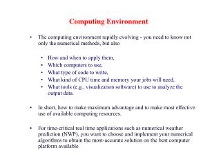
1. Computing Environment • The computing environment rapidly evolving ‑ you need to know not only the numerical methods, but also  • How and when to apply them, • Which computers to use, • What type of code to write, • What kind of CPU time and memory your jobs will need, • What tools (e.g., visualization software) to use to analyze the output data. • In short, how to make maximum advantage and to make most effective use of available computing resources. • For time-critical real time applications such as numerical weather prediction (NWP), you want to choose and implement your numerical algorithms to obtain the most-accurate solution on the best computer platform available

2. Definitions – Clock Cycles, Clock Speed • Computer chip operates at discrete intervals called clocks. Often measured in nanoseconds (ns) or megahertz. • 3200 megaHz (MHz) = 3.2 GigaHz (GHz) (fastest Pentium IV as of today) ~ clock speed of 0.3 nanosecond (ns) • 100 mhz (Cray J90 vector processor) -> 10 ns (an OU computer retired earlier this year) • May take several clocks to do one multiplication • Memory access also takes time, not just computation • mHz is not the only measure of CPU speed. Different CPUs of the same mHz often differ in speed. E.g., the 1.5GHz Itanium 2, Intel’s latest 64bit processor, is much faster than the 3.2GHz Pentium V.

3. Definitions – FLOPS • Floating Operations / Second • Megaflops – million FLOPS • Gigaflops – billion FLOPS • Teraflops – trillion FLOPS • A good measure of code performance – typically one add is one flop, one multiplication is also on flop • Cray J90 Vector theoretical peak speed = 200 Mflops, most codes achieves only 1/3 of peak • Fastest US-made vector CPU - Cray T90 peak = 3.2 Gflops • NEC XS-5 Vector CPU Used in Earth Simulation (by far the fastest computer in the world right now) = 8 Gflops • Fastest Super-scalar Processors of today include HP Alpha, IBM Power 4 and Intel Itanium 2 processors, have peak speed of several GFLOPS • See http://www.specbench.org for the latest benchmarks of processors for real world problems. Specbench numbers are relative.

4. MIPS • Million instructions per second – also a measure of computer speed – used most the old days when computer architectures were relatively simple • MIPS is hardly used these days because the number of instructions used to complete one FLOP is very much CPU dependent with today’s CPUS

5. What’s an Instruction? • Load a value from a specific address in main memory into a specific register • Store a value from a specific register into a specific address in main memory • Add two specific registers together and put their sum in a specific register – or subtract, multiply, divide, square root, etc • Determine whether two registers both contain nonzero values (“AND”) • Jump from one sequence of instructions to another (branch) • … and so on

6. Bandwidth • The speed at which data flow across a network or wire • 56K Modem = 56 kilobits / second • T1 link = 1.554 mbits / sec • T3 link = 45 mbits / sec • FDDI = 100 mbits / sec • Fiber Channel = 800 mbits /sec • 100 BaseT (fast) Ethernet = 100 mbits/ sec • Gigabit Ethernet = 1000 mbits /sec • Brain system = 3 Gbits / s • 1 bytes = 8 bits

7. Central Processing Unit • Also called CPU or processor: the “brain” • Parts • Control Unit: figures out what to do next -- e.g., whether to load data from memory, or to add two values together, or to store data into memory, or to decide which of two possible actions to perform (branching) • Arithmetic/Logic Unit: performs calculations – e.g., adding, multiplying, checking whether two values are equal • Registers: where data reside that are being used right now

8. Hardware Evolution • Mainframe computers • Vector Supercomputers • Workstations • Microcomputers / Personal Computers • Desktop Supercomputers • Workstation Super Clusters • Supercomputer Clusters • Handheld, Palmtop, Calculators, • et al….

9. Types of Processors • Scalar (Serial) • One operation per clock cycle • Vector • Multiple operations per clock cycle. Typically achieved at the loop level where the instructions are the same or similar for each loop index • Superscalar (most of today’s microprocessors) • Several operations per clock cycle

10. Types of Computer Systems • Single Processor Scalar (e.g., ENIAC, IBM704, traditional IBM-PC and Mac) • Single Processor Vector (CDC7600, Cray-1) • Multi-Processor Vector (e.g., Cray XMP, Cray C90, Cray J90, NEC SX-5), • Single Processor Super-scalar (Sun Sparc Workstations) • Multi-processor scalar (e.g., Multi-processor Pentium PC) • Multi-processor super-scalar (e.g., SOM Sun Enterprise Server Rossby, IBM Regata of OSCER Sooner, SGI Origin 2000 of CAPS Paige) • Clusters of the above (e.g., OSCER Linux clusters Boomer – cluster of 2-CPU Pentium IV Linux Workstations, Earth Simulator – Cluster of multiple vector processor nodes)

11. ENIAC – World’s first electronic computer (1946-1955) • The world's first electronic digital computer, Electronic Numerical Integrator and Computer (ENIAC), was developed by Army Ordnance to compute World War II ballistic firing tables. • ENIAC’s thirty separate units, plus power supply and forced-air cooling, weighed over thirty tons. It had 19,000 vacuum tubes, 1,500 relays, and hundreds of thousands of resistors, capacitors, and inductors and consumed almost 200 kilowatts of electrical power. • See story at http://ftp.arl.mil/~mike/comphist/eniac-story.html

12. ENIAC – World’s first electronic computer (1946-1955) Fromhttp://ftp.arl.army.mil/ftp/historic-computers

13. ENIAC – World’s first electronic computer (1946-1955) From http://ftp.arl.army.mil/ftp/historic-computers

14. Cray-1, the first ‘vector supercomputer’, 1976 • Single vector processor • 133 MFLOPS peak speed • 1 million 8 byte words = 8mb of memory • Price $5-8 million • Liquid cooling system using Freon • Right – Cray 1A on exhibit at NCAR

15. Cray-J90 • Air-cooled, low-cost vector supercomputers introduced by Cray in the mid-'90s. • OU owned a 16-processor J90. Not decommissioned until early 2003.

16. Cray-T90, the last major shared-memory parallel vector supercomputer made by US Company • Up to 32 vector processors • 1.76 GFLOPS/CPU • 512MW = 4 GB memory • Decommissioned from San Diego Supercomputer Center in March 2002 • See Historic Cray Systems at http://136.162.32.160/company/h_systems.html

17. Memory Architectures • Shared Memory Parallel (SMP) Systems • Distributed Memory Parallel (DMP) Systems • Memory can be accessed and addressed • uniformly by all processors with no user intervention • Fast/expensive CPU, Memory, and networks • Easier to use • Difficult to scale to many (> 32) processors • Each processor has its own memory • Others can access its memory only via • network communications • Often off-the-shelf components, • therefore low cost • Harder to use, explicit user specification of • communications often needed. • Not suitable for inherently serial codes • High-scalability - largest current system • has nearly many thousands of processors

18. Memory Architectures • Multi-level memory (cache and main memory) architectures • Cache – fast and expensive memory • Typical L1 cache size in current day microprocessors ~ 32 K • L2 size ~ 256K to 8mb (P4 has 512K) • Main memory a few Mb to many Gb. • Try to reuse the content of cache as much as possible before the content is replaced by new data or instructions • Disk, CD ROM etc – the slowest forms of memory – still direct access • Tapes, even slower, serial access only Disk etc

19. OSCER Hardware: IBM Regatta 32 Power4 CPUs 32 GB RAM 200 GB disk OS: AIX 5.1 Peak speed: 140 billion calculations per second Programming model: shared memory multithreading

20. OSCER IBM Regatta p690 Specs – sooner.ou.edu • 32 Power4 processors running at 1.1 GHz • 32 GB shared memory. Distributed memory parallelization is also supported via message passing (MPI) • 3 levels of cache. 32KB L1 cache per CPU, 1.41MB L2 cache shared by each two CPUs, and 128mb L3 cache shared by eight processors. • The peak performance of each processor is 4.4 GFLOPS (4 FLOPS per cycle). • See also http://www.oscer.ou.edu/hardsoft_ibm_regatta_p690.html for additional information

21. IBM p-Series server (sooner) architecture(from http://www.redbooks.ibm.com/pubs/pdfs/redbooks/sg247041.pdf)

22. IBM p-Series server (sooner) architecture

23. OSCER Hardware: Linux Cluster 264 Pentium4 CPUs 264 GB RAM 2.5 TB disk OS: Red Hat Linux 7.3 Peak speed: over a trillion calculations per second Programming model: distributed multiprocessing

24. OSCER Linux cluster specs – boomer.ou.edu • Intel Pentium-4 Xeon DP processors running at 2.0 GHz • Each node contains 2 CPUs, each node has 2GB memory • Each processor has 512K L-2 cache • Interconnet: Myrinet (primary) and 100Mbps Ethernet (backup) • Total theoretical peak performance 1.08 Teraflops • System: Linux 7.3 • See also http://www.oscer.ou.edu/hardsoft_aspen_cluster_pentium4.html for additional information

25. SOM Metlab Workstations • Dell dual-processor capable 530 Workstations (metlab1.ou.edu through metlab25.ou.edu) • Configured with single Intel 1.7GHz Pentium 4 Xeon processors and 1GB memory • 100Mbps Ethernet • Not set up to run MPI jobs but can be • Fortran compilers available: g77 and Intel Fortran ifc (version 6.0) • The workstations are not logged in most of the time (who and top commands show who are logged in and the running processes on the machine)!

26. Parallelism • Parallelism means doing multiple things at the same time: you can get more work done in the same time.

27. Instruction Level Parallelization • Superscalar: perform multiple operations at the same time • Pipeline: start performing an operation on one piece of data while finishing the same operation on another piece of data • Superpipeline: perform multiple pipelined operations at the same time • Vector: load multiple pieces of data into special registers in the CPU and perform the same operation on all of them at the same time

28. What’s an Instruction? • Load a value from a specific address in main memory into a specific register • Store a value from a specific register into a specific address in main memory • Add two specific registers together and put their sum in a specific register – or subtract, multiply, divide, square root, etc • Determine whether two registers both contain nonzero values (“AND”) • Jump from one sequence of instructions to another (branch) • … and so on

29. Scalar Operation z = a * b + c * d • Loadainto registerR0 • LoadbintoR1 • MultiplyR2 = R0 * R1 • LoadcintoR3 • LoaddintoR4 • MultiplyR5 = R3 * R4 • AddR6 = R2 + R5 • StoreR6intoz How would this statement be executed?

30. Does Order Matter? z = a * b + c * d • LoadaintoR0 • LoadbintoR1 • MultiplyR2 = R0 * R1 • LoadcintoR3 • LoaddintoR4 • MultiplyR5 = R3 * R4 • AddR6 = R2 + R5 • StoreR6intoz LoaddintoR4 LoadcintoR3 MultiplyR5 = R3 * R4 LoadaintoR0 LoadbintoR1 MultiplyR2 = R0 * R1 AddR6 = R2 + R5 StoreR6intoz In the cases where order doesn’t matter, we say that the operations are independent of one another.

31. Superscalar Operation z = a * b + c * d • LoadaintoR0 ANDloadbintoR1 • MultiplyR2 = R0 * R1 ANDloadcintoR3 AND loaddintoR4 • MultiplyR5 = R3 * R4 • AddR6 = R2 + R5 • StoreR6intoz So, we go from 8 operations down to 5.

32. Superscalar Loops DO i = 1, n z(i) = a(i)*b(i) + c(i)*d(i) END DO !! i = 1, n Each of the iterations is completely independent of all of the other iterations; e.g., z(1) = a(1)*b(1) + c(1)*d(1) has nothing to do with z(2) = a(2)*b(2) + c(2)*d(2) Operations that are independent of each other can be performed in parallel.

33. Superscalar Loops for (i = 0; i < n; i++) { z[i] = a[i]*b[i] + c[i]*d[i]; } /* for i */ • Loada[i]intoR0ANDloadb[i]intoR1 • Multiply R2 = R0 * R1 ANDload c[i] into R3 ANDload d[i] into R4 • Multiply R5 = R3 * R4 ANDload a[i+1] into R0 ANDload b[i+1] into R1 • Add R6 = R2 + R5 ANDloadc[i+1]intoR3ANDloadd[i+1]intoR4 • StoreR6intoz[i]ANDmultiplyR2 = R0 * R1 • etc etc etc

34. Example: IBM Power4 8-way Superscalar: can execute up to 8 operations at the same time[12] • 2 integer arithmetic or logical operations, and • 2 floating point arithmetic operations, and • 2 memory access (load or store) operations, and • 1 branch operation, and • 1 conditional operation

35. Pipelining Pipelining is like an assembly line or a bucket brigade. • An operation consists of multiple stages. • After a set of operands complete a particular stage, they move into the next stage. • Then, another set of operands can move into the stage that was just abandoned.

36. Instruction Fetch Instruction Fetch Instruction Fetch Instruction Fetch Instruction Decode Instruction Decode Instruction Decode Instruction Decode Operand Fetch Operand Fetch Operand Fetch Operand Fetch Instruction Execution Instruction Execution Instruction Execution Instruction Execution Result Writeback Result Writeback Result Writeback Result Writeback Pipelining Example t = 2 t = 5 t = 0 t = 1 t = 3 t = 4 t = 6 t = 7 i = 1 i = 2 i = 3 i = 4 Computation time If each stage takes, say, one CPU cycle, then once the loop gets going, each iteration of the loop only increases the total time by one cycle. So a loop of length 1000 takes only 1004 cycles. [13]

37. Superpipelining Superpipelining is a combination of superscalar and pipelining. So, a superpipeline is a collection of multiple pipelines that can operate simultaneously. In other words, several different operations can execute simultaneously, and each of these operations can be broken into stages, each of which is filled all the time. So you can get multiple operations per CPU cycle. For example, a IBM Power4 can have over 200 different operations “in flight” at the same time.[12]

38. Vector Processing • The most power CPU or processors (e.g., Cray T90 and NEC SX-5) are vector processors that can perform operations on a stream of data in a pipelined fashion – so vectorization is one type of pipelining. • A vector here is defined as an ordered list of scalar values. For example, an array stored in memory is a vector. • Vector systems have machine instructions (vector instructions) that fetch a vector of values (instead of single ones) from memory, operate on them and store them back to memory. • Basically, vector processing is a version of the Single Instruction Multiple Data (SIMD) parallel processing technique. • On the other hand, scalar processing usually requires one instruction to act on each data value.

39. Vector Processing - Example DO I = 1, N A(I) = B(I) + C(I) ENDDO • If the above code is vectorized, the following processes will take place, • A vector of values in B(I) will be fetched from memory. • A vector of values in C(I) will be fetched from memory. • A vector add instruction will operate on pairs of B(I) and C(I) values. • After a short start-up time, stream of A(I) values will be stored back to memory, one value every clock cycle. • If the code is not vectorized, the following scalar processes will take place, • B(1) will be fetched from memory. • C(1) will be fetched from memory. • A scalar add instruction will operate on B(1) and C(1). • A(1) will be stored back to memory • Step (1) to (4) will be repeated N times.

40. Vector Processing • Vector processing allows a vector of values to be fed continuously to the vector processor. • If the value of N is large enough to make the start-up time negligible in comparison, on the average the vector processor is capable of producing close to one result per clock cycle (imaging the automobile assembly line)

41. Vector Processing • If the same code is not vectorized (using J90 as an example), for every I iteration, e.g. I=1, a clock cycle each is needed to fetch B(1) and C(1), about 4 clock cycles are needed to complete a floating-point add operation, and another clock cycle is needed to store the value A(1). • Thus a minimum of 6 clock cyclesare needed to produce one result (complete one iterations). • We can say that there is a speed up of about 6 times for this example if the code is vectorized.

42. Vector Processing • Vector processors can often chain operations such as add and multiplication together (because they have multiple functional units, for add, multiply etc), in much the same way as superscalar processor does, so that both operations can be done in one clock cycles. This further increases the processing speed. • It usually helps to have long statements inside vector loops in this case.

43. Vectorization for Vector Computers • Characteristics of Vectorizable Code • Vectorization can only be done within a DO loop, and it must be the innermost DO loop (unless loops at different levels are merged together by the compiler). • There need to be sufficient iterations in the DO loop to offset the start-up time overhead. • Try to put more work into a vectorizable statement (by having more operations) to provide more opportunities for concurrent operation (However, the compiler may not vectorize a loop if it is too complicated).

44. Vectorization for Vector Computers • Vectorization Inhibitors • Recursive data dependencies is one of the most 'destructive' vectorization inhibitors. E.g., A(I) = A(I-1) + B(I) • Subroutine calls, • References to external functions • input/output statements • Assigned GOTO statements • Certain nested IF blocks and backward transfers within loops.

45. Vectorization for Vector Computers • Inhibitors such as subroutine or function calls inside loop can be removed by expanding the function or inlining subroutine at the point of reference. • Vectorization Directive – compiler directives can be manually inserted into code to force or prevent vectorization of specific loops • Most of the loop vectorizations can be achieved automatically by compilers with proper option. • Although true vector processors (e.g., Cray processors) has become few, limited vector support has recently been incorporated into super-scalar processors such as Pentium 4 and PowerPC processors used in PowerMac. • Code that vectorizes well generally also performs well on super-scalar processors since the latter also exploits pipeline parallelidm in the program

46. Amhdal’s Law • Amhdal’s Law (1967): where a is the time needed for the serial portion of the task. When Napproaches infinity, speedup = 1/ a.

47. Message Passing for DMP • Messaging Passing Interface (MPI) has emerged as the standard for parallel programming on distributed-memory parallel systems • MPI is essentially a library of subroutines that handle data exchanges between programs running on different nodes • Domain decomposition is the commonly used strategy for distributing data and computations among nodes

48. Domain Decomposition Strategy in ARPS • Spatial domain decomposition of ARPS grid. • Each square in the upper panel corresponds to a single processor with its own memory. • The lower panel details a single processor. Grid points having a white background are updated without communication, while those in dark stippling require information from neighboring processors. • To avoid communication in the latter, data from the outer border of neighboring processors (light stippling) are stored locally.

49. Performance of the ARPS on various computing platforms. The ARPS is executed using a 19x19x43 km grid per processor such that the overall grid domain increases proportionally as the number of processors increase. For a perfect system, the run time should not increase as processors are added, which would results in a line of zero slope.

50. Issues with Parallel Computing • Load-balance / Synchronization • Try to give equal amount of workload to each processor • Try to give processors that finish first more work to do (load rebalance) • The goal is to keep all processors as busy as possible • Communication / Locality • Inter-processor or internode communications typically the largest overhead on distributed-memory platforms, because network is slow relative to CPU speed • Try to keep data access local • E.g., 2nd-order finite difference requires data at 3 points 4th-order finite difference requires data at 5 points